Vector multiplication in python

Работа с векторами в Python с помощью NumPy

В этом уроке мы узнаем, как создать вектор с помощью библиотеки Numpy в Python. Мы также рассмотрим основные операции с векторами, такие как сложение, вычитание, деление и умножение двух векторов, векторное точечное произведение и векторное скалярное произведение.

Что такое вектор в Python?

Вектор известен как одномерный массив. Вектор в Python – это единственный одномерный массив списков, который ведет себя так же, как список Python. Согласно Google, вектор представляет направление, а также величину; особенно он определяет положение одной точки в пространстве относительно другой.

Векторы очень важны в машинном обучении, потому что у них есть величина, а также особенности направления. Давайте разберемся, как мы можем создать вектор на Python.

Создание вектора в Python

Модуль Python Numpy предоставляет метод numpy.array(), который создает одномерный массив, то есть вектор. Вектор может быть горизонтальным или вертикальным.

Вышеупомянутый метод принимает список в качестве аргумента и возвращает numpy.ndarray.

Давайте разберемся в следующих примерах.

Пример – 1: горизонтальный вектор

# Importing numpy import numpy as np # creating list list1 = [10, 20, 30, 40, 50] # Creating 1-D Horizontal Array vtr = np.array(list1) vtr = np.array(list1) print("We create a vector from a list:") print(vtr)

We create a vector from a list: [10 20 30 40 50]

Пример – 2: Вертикальный вектор

# Importing numpy import numpy as np # defining list list1 = [[12], [40], [6], [10]] # Creating 1-D Vertical Array vtr = np.array(list1) vtr = np.array(list1) print("We create a vector from a list:") print(vtr)

We create a vector from a list: [[12] [40] [ 6] [10]]

Базовые операции вектора Python

После создания вектора мы теперь будем выполнять арифметические операции над векторами.

Ниже приведен список основных операций, которые мы можем производить с векторами:

• сложение;
• вычитание;
• умножение;
• деление;
• точечное произведение;
• скалярные умножения.

Сложение двух векторов

В векторном сложении это происходит поэлементно, что означает, что сложение будет происходить поэлементно, а длина будет такой же, как у двух аддитивных векторов.

Давайте разберемся в следующем примере.

import numpy as np list1 = [10,20,30,40,50] list2 = [11,12,13,14,15] vtr1 = np.array(list1) vtr2= np.array(list2) print("We create vector from a list 1:") print(vtr1) print("We create vector from a list 2:") print(vtr2) vctr_add = vctr1+vctr2 print("Addition of two vectors: ",vtr_add)

We create vector from a list 1: [10 20 30 40 50] We create vector from a list 2: [11 12 13 14 15] Addition of two vectors: [21 32 43 54 65]

Вычитание

Вычитание векторов выполняется так же, как и сложение, оно следует поэлементному подходу, и элементы вектора 2 будут вычтены из вектора 1. Давайте разберемся в следующем примере.

import numpy as np list1 = [10,20,30,40,50] list2 = [5,2,4,3,1] vtr1 = np.array(list1) vtr2= np.array(list2) print("We create vector from a list 1:") print(vtr1) print("We create a vector from a list 2:") print(vtr2) vtr_sub = vtr1-vtr2 print("Subtraction of two vectors: ",vtr_sub)

We create vector from a list 1: [10 20 30 40 50] We create vector from a list 2: [5 2 4 3 1] Subtraction of two vectors: [5 18 26 37 49]

Умножение векторов

Элементы вектора 1 умножаются на вектор 2 и возвращают векторы той же длины, что и векторы умножения.

import numpy as np list1 = [10,20,30,40,50] list2 = [5,2,4,3,1] vtr1 = np.array(list1) vtr2= np.array(list2) print("We create vector from a list 1:") print(vtr1) print("We create a vector from a list 2:") print(vtr2) vtr_mul = vtr1*vtr2 print("Multiplication of two vectors: ",vtr_mul)

We create vector from a list 1: [10 20 30 40 50] We create vector from a list 2: [5 2 4 3 1] Multiplication of two vectors: [ 50 40 120 120 50]

Умножение производится следующим образом.

vct[0] = x[0] * y[0] vct[1] = x[1] * y[1]

Первый элемент вектора 1 умножается на первый элемент соответствующего вектора 2 и так далее.

Операция деления двух векторов

В операции деления результирующий вектор содержит значение частного, полученное при делении двух элементов вектора.

Давайте разберемся в следующем примере.

import numpy as np list1 = [10,20,30,40,50] list2 = [5,2,4,3,1] vtr1 = np.array(list1) vtr2= np.array(list2) print("We create vector from a list 1:") print(vtr1) print("We create a vector from a list 2:") print(vtr2) vtr_div = vtr1/vtr2 print("Division of two vectors: ",vtr_div)

We create vector from a list 1: [10 20 30 40 50] We create vector from a list 2: [5 2 4 3 1] Division of two vectors: [ 2. 10. 7.5 13.33333333 50. ]

Как видно из вышеприведенного вывода, операция деления вернула частное значение элементов.

Векторное точечное произведение

Векторное скалярное произведение выполняется между двумя последовательными векторами одинаковой длины и возвращает единичное скалярное произведение. Мы будем использовать метод .dot() для выполнения скалярного произведения. Это произойдет, как показано ниже.

vector c = x . y =(x1 * y1 + x2 * y2)

Давайте разберемся в следующем примере.

import numpy as np list1 = [10,20,30,40,50] list2 = [5,2,4,3,1] vtr1 = np.array(list1) vtr2= np.array(list2) print("We create vector from a list 1:") print(vtr1) print("We create a vector from a list 2:") print(vtr2) vtr_product = vtr1.dot(vtr2) print("Dot product of two vectors: ",vtr_product)

We create vector from a list 1: [10 20 30 40 50] We create vector from a list 2: [5 2 4 3 1] Dot product of two vectors: 380

Векторно-скалярное умножение

В операции скалярного умножения; мы умножаем скаляр на каждую компоненту вектора. Давайте разберемся в следующем примере.

import numpy as np list1 = [10,20,30,40,50] vtr1 = np.array(list1) scalar_value = 5 print("We create vector from a list 1:") print(vtr1) # printing scalar value print("Scalar Value : " + str(scalar_value)) vtr_scalar = vtr1 * scalar_value print("Multiplication of two vectors: ",vtr_scalar)

We create vector from a list 1: [10 20 30 40 50] Scalar Value : 5 Multiplication of two vectors: [ 50 100 150 200 250]

В приведенном выше коде скалярное значение умножается на каждый элемент вектора в порядке s * v =(s * v1, s * v2, s * v3).

Источник

Introduction

The dot product is a major concept of linear algebra and thus machine learning and data science. We will see some properties of this operation. Then, we will get some intuition on the link between matrices and systems of linear equations.

2.2 Multiplying Matrices and Vectors

The standard way to multiply matrices is not to multiply each element of one with each element of the other (called the element-wise product) but to calculate the sum of the products between rows and columns. The matrix product, also called dot product, is calculated as following:

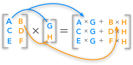
The dot product between a matrix and a vector

The number of columns of the first matrix must be equal to the number of rows of the second matrix. If the dimensions of the first matrix is ($m \times n$), the second matrix needs to be of shape ($n \times x$). The resulting matrix will have the shape ($m \times x$).

Example 1.

Let’s start with the multiplication of a matrix and a vector.

We saw that the formula is the following:

$ \begin &\begin 1 & 2 \\ 3 & 4 \\ 5 & 6 \end\times \begin 2 \\ 4 \end=\\ &\begin 1 \times 2 + 2 \times 4 \\ 3 \times 2 + 4 \times 4 \\ 5 \times 2 + 6 \times 4 \end= \begin 10 \\ 22 \\ 34 \end \end $

It is a good habit to check the dimensions of the matrix to see what is going on. We can see in this example that the shape of $\bs$ is ($3 \times 2$) and the shape of $\bs$ is ($2 \times 1$). So the dimensions of $\bs$ are ($3 \times 1$).

With Numpy

The Numpy function dot() can be used to compute the matrix product (or dot product). Let’s try to reproduce the last exemple:

It is equivalent to use the method dot() of Numpy arrays:

Example 2.

Multiplication of two matrices.

$\bs=\begin 2 & 7 \\ 1 & 2 \\ 3 & 6 \end $

$ \begin &\begin 1 & 2 & 3 \\ 4 & 5 & 6 \\ 7 & 8 & 9 \\ 10 & 11 & 12 \end \begin 2 & 7 \\ 1 & 2 \\ 3 & 6 \end=\\ &\begin 2 \times 1 + 1 \times 2 + 3 \times 3 & 7 \times 1 + 2 \times 2 + 6 \times 3 \\ 2 \times 4 + 1 \times 5 + 3 \times 6 & 7 \times 4 + 2 \times 5 + 6 \times 6 \\ 2 \times 7 + 1 \times 8 + 3 \times 9 & 7 \times 7 + 2 \times 8 + 6 \times 9 \\ 2 \times 10 + 1 \times 11 + 3 \times 12 & 7 \times 10 + 2 \times 11 + 6 \times 12 \\ \end\\ &= \begin 13 & 29 \\ 31 & 74 \\ 49 & 119 \\ 67 & 164 \end \end $

Let’s check the result with Numpy:

A = np.array([[1, 2, 3], [4, 5, 6], [7, 8, 9], [10, 11, 12]]) A 

array([[ 1, 2, 3], [ 4, 5, 6], [ 7, 8, 9], [10, 11, 12]])

array([[ 13, 29], [ 31, 74], [ 49, 119], [ 67, 164]])

Formalization of the dot product

The dot product can be formalized through the following equation:

You can find more examples about the dot product here.

Properties of the dot product

We will now see some interesting properties of the dot product. Using simple examples for each property, we’ll get used to the Numpy functions.

Simplification of the matrix product

Matrix mutliplication is distributive

Example 3.

Matrix mutliplication is associative

Matrix multiplication is not commutative

However vector multiplication is commutative

Let’s try with the following example:

One way to see why the vector multiplication is commutative is to notice that the result of $\bs>y>$ is a scalar. We know that scalars are equal to their own transpose, so mathematically, we have:

System of linear equations

This is an important part of why linear algebra can be very useful to solve a large variety of problems. Here we will see that it can be used to represent systems of equations.

A system of equations is a set of multiple equations (at least 1). For instance we could have:

$ \begin y = 2x + 1 \\ y = \fracx +3 \end $

It is defined by its number of equations and its number of unknowns. In this example, there are 2 equations (the first and the second line) and 2 unknowns ($x$ and $y$). In addition we call this a system of linear equations because each equation is linear. We can represent that in 2 dimensions: we have one straight line per equation and dimensions correspond to the unknowns. Here is the plot of the first equation:

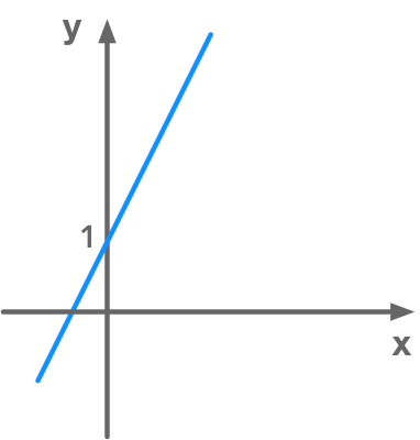
Representation of a linear equation

In our system of equations, the unknowns are the dimensions and the number of equations is the number of lines (in 2D) or $n$-dimensional planes.

Using matrices to describe the system

Matrices can be used to describe a system of linear equations of the form $\bs=\bs$. Here is such a system:

$ A_x_1 + A_x_2 + A_x_n = b_1 \\ A_x_1 + A_x_2 + A_x_n = b_2 \\ \cdots \\ A_x_1 + A_x_2 + A_x_n = b_n $

The unknowns (what we want to find to solve the system) are the variables $x_1$ and $x_2$. It is exactly the same form as with the last example but with all the variables on the same side. $y = 2x + 1$ becomes $-2x + y = 1$ with $x$ corresponding to $x_1$ and $y$ corresponding to $x_2$. We will have $n$ unknowns and $m$ equations.

The variables are named $x_1, x_2, \cdots, x_n$ by convention because we will see that it can be summarised in the vector $\bs$.

Left-hand side

with a vector $\bs$ containing the $n$ unknowns

$ \bs= \begin x_1 \\ x_2 \\ \cdots \\ x_n \end $

Matrix form of a system of linear equations

We have a set of two equations with two unknowns. So the number of rows of $\bs$ gives the number of equations and the number of columns gives the number of unknowns.

Both sides

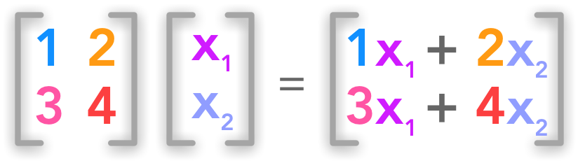
The equation system can be wrote like that:

$ \begin A_ & A_ & \cdots & A_ \\ A_ & A_ & \cdots & A_ \\ \cdots & \cdots & \cdots & \cdots \\ A_ & A_ & \cdots & A_ \end \begin x_1 \\ x_2 \\ \cdots \\ x_n \end = \begin b_1 \\ b_2 \\ \cdots \\ b_m \end $

Example 4.

We will try to convert the common form of a linear equation $y=ax+b$ to the matrix form. If we want to keep the previous notation we will have instead:

Don’t confuse the variable $x_1$ and $x_2$ with the vector $\bs$. This vector contains all the variables of our equations:

In this example we will use the following equation:

$ \begin &x_2=2x_1+1 \\ \Leftrightarrow& 2x_1-x_2=-1 \end $

To complete the equation we have

This system of equations is thus very simple and contains only 1 equation ($\bs$ has 1 row) and 2 variables ($\bs$ has 2 columns).

We will see at the end of the the next chapter that this compact way of writing sets of linear equations can be very usefull. It provides a way to solve the equations.

References

Feel free to drop me an email or a comment. The syllabus of this series can be found in the introduction post. All the notebooks can be found on Github.

Источник