Total least squares python

Python total_least_squares Example

The python total_least_squares example is extracted from the most popular open source projects, you can refer to the following example for usage. Programming language: Python Namespace/package name: agpyfit_a_line

 v = np.array([x.value/1000. for x in leaf_vrms[leaf]]) pl.plot(r, v, linestyle='-', marker=markers.next(), alpha=0.5, color=color) trunkslopes = <> xvals = <> # filter based on minimum radius in arcsec min_rad_as = 15 for trunk in trunk_leaves: if trunk_leaves[trunk][0] in leaf_stats: # size-linewidth -> sigma=0.72 R^0.5 x = [(j.value*as_to_pc)**0.5 for leaf in trunk_leaves[trunk] for j in leaf_radii[leaf] if j.value > min_rad_as] y = [j.value/1000. for leaf in trunk_leaves[trunk] for j,r in zip(leaf_vrms[leaf],leaf_radii[leaf]) if r.value > min_rad_as] if len(x) $ (pc at D=7.5 kpc)") pl.ylabel(r'$\sigma_v$ (km s$^$') pl.title(r'$\sigma_v = C R^$, $C>1.4$ or $C<0.35$') pl.plot(np.linspace(0,5)**0.5,0.72*np.linspace(0,5)**0.5,'k--',linewidth=2,alpha=0.5) pl.figure(5) pl.clf() pl.xlabel("R$^$ (pc at D=7.5 kpc)") pl.ylabel(r'$\sigma_v$ (km s$^$') pl.title(r'$\sigma_v = C R^$, $C\sim0.7$') pl.plot(np.linspace(0,5)**0.5,0.72*np.linspace(0,5)**0.5,'k--',linewidth=2,alpha=0.5)

 continue print mp.axis_number(ypos[yd], xpos[xd]), xpos[xd], ypos[yd] ax = mp.grid[mp.axis_number(ypos[yd], xpos[xd])] # ax.plot(data[xd][rrlmask],data[yd][rrlmask],'.') mpl_plot_templates.adaptive_param_plot( data[xd][rrlmask].to(u.Jy).value, data[yd][rrlmask].to(u.Jy).value, bins=30, threshold=5, fill=False, alpha=0.8, axis=ax, cmap=pl.mpl.cm.spectral, ) axlims = ax.axis() factor = fit_a_line.total_least_squares(data[xd][rrlmask], data[yd][rrlmask], intercept=False) ax.plot(np.linspace(0, 20), factor * np.linspace(0, 20), "k--", linewidth=2, alpha=0.5, label="$y=%0.2fx$" % factor) ax.axis(axlims) # reset plot limits ax.legend(loc="best", fontsize=16) # tweaks to prevent tick overlaps if xpos[xd] > 0: ax.set_yticklabels([]) ax.set_ylabel("") else: ax.set_ylabel(yd) ax.set_xlabel(xd) if ypos[yd] > 0: ax.set_yticks(ax.get_yticks()[:-1]) # if ypos[yd] == 2:

cont11 = fits.getdata(cont11filename) cont22 = fits.getdata(cont22filename) rrlerr6cm = 0.0415 rrlerr2cm = 0.0065 rrl6cmmask = rrl6cm > rrlerr6cm * 2 rrl2cmmask = rrl2cm > rrlerr2cm * 2 offset2cm, offset6cm = 0,0 rrldata,contdata,rrlmask = (rrl2cm,cont22,rrl2cmmask) rrlmask *= (contdata > 0.1) nok = np.count_nonzero(rrlmask) factor2cm,offset2cm = fit_a_line.total_least_squares(rrldata[rrlmask], contdata[rrlmask], data1err=np.ones(nok)*rrlerr2cm, data2err=np.ones(nok)*0.05, print_results=True, intercept=True) print "2cm: ",offset2cm,factor2cm artificial_cont_2cm = rrldata * factor2cm + offset2cm rrldata,contdata,rrlmask = (rrl6cm,cont11,rrl6cmmask) rrlmask *= (contdata > 0.1) nok = np.count_nonzero(rrlmask) factor6cm, offset6cm = fit_a_line.total_least_squares(rrldata[rrlmask], contdata[rrlmask], data1err=np.ones(nok)*rrlerr6cm, data2err=np.ones(nok)*0.05, print_results=True, intercept=True)

Related

• Python KSSPlugin Example
• Python MonyPlugin Example
• Python Feedpoller Example
• Python RenameExtension Example
• Python SyncMode Example
• Python DictionaryEditor Example
• Python IMissionReport Example
• Python IStatusUpdate Example
• Python IUserProfile Example
• Python IRightColumn Example
• Python IManagedLDAPPlugin Example
• Python ZipFileImportContext Example
• Python IPortletManagerMenu Example
• Python AngularAppPortalRootTraverser Example
• Python InferenceAgent Example
• Python FrameSamplingFilter Example

Источник

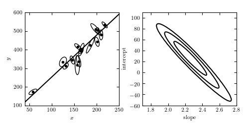
Total Least Squares Figure¶

A linear fit to data with correlated errors in x and y. In the literature, this is often referred to as total least squares or errors-in-variables fitting. The left panel shows the lines of best fit; the right panel shows the likelihood contours in slope/intercept space. The points are the same set used for the examples in Hogg, Bovy & Lang 2010.

Code output:

Optimization terminated successfully. Current function value: 55.711167 Iterations: 88 Function evaluations: 164 

Python source code:

# Author: Jake VanderPlas # License: BSD # The figure produced by this code is published in the textbook # "Statistics, Data Mining, and Machine Learning in Astronomy" (2013) # For more information, see http://astroML.github.com # To report a bug or issue, use the following forum: # https://groups.google.com/forum/#!forum/astroml-general import numpy as np from scipy import optimize from matplotlib import pyplot as plt from matplotlib.patches import Ellipse from astroML.linear_model import TLS_logL from astroML.plotting.mcmc import convert_to_stdev from astroML.datasets import fetch_hogg2010test #---------------------------------------------------------------------- # This function adjusts matplotlib settings for a uniform feel in the textbook. # Note that with usetex=True, fonts are rendered with LaTeX. This may # result in an error if LaTeX is not installed on your system. In that case, # you can set usetex to False. if "setup_text_plots" not in globals(): from astroML.plotting import setup_text_plots setup_text_plots(fontsize=8, usetex=True) #------------------------------------------------------------ # Define some convenience functions # translate between typical slope-intercept representation, # and the normal vector representation def get_m_b(beta): b = np.dot(beta, beta) / beta[1] m = -beta[0] / beta[1] return m, b def get_beta(m, b): denom = (1 + m * m) return np.array([-b * m / denom, b / denom]) # compute the ellipse pricipal axes and rotation from covariance def get_principal(sigma_x, sigma_y, rho_xy): sigma_xy2 = rho_xy * sigma_x * sigma_y alpha = 0.5 * np.arctan2(2 * sigma_xy2, (sigma_x ** 2 - sigma_y ** 2)) tmp1 = 0.5 * (sigma_x ** 2 + sigma_y ** 2) tmp2 = np.sqrt(0.25 * (sigma_x ** 2 - sigma_y ** 2) ** 2 + sigma_xy2 ** 2) return np.sqrt(tmp1 + tmp2), np.sqrt(tmp1 - tmp2), alpha # plot ellipses def plot_ellipses(x, y, sigma_x, sigma_y, rho_xy, factor=2, ax=None): if ax is None: ax = plt.gca() sigma1, sigma2, alpha = get_principal(sigma_x, sigma_y, rho_xy) for i in range(len(x)): ax.add_patch(Ellipse((x[i], y[i]), factor * sigma1[i], factor * sigma2[i], alpha[i] * 180. / np.pi, fc='none', ec='k')) #------------------------------------------------------------ # We'll use the data from table 1 of Hogg et al. 2010 data = fetch_hogg2010test() data = data[5:] # no outliers x = data['x'] y = data['y'] sigma_x = data['sigma_x'] sigma_y = data['sigma_y'] rho_xy = data['rho_xy'] #------------------------------------------------------------ # Find best-fit parameters X = np.vstack((x, y)).T dX = np.zeros((len(x), 2, 2)) dX[:, 0, 0] = sigma_x ** 2 dX[:, 1, 1] = sigma_y ** 2 dX[:, 0, 1] = dX[:, 1, 0] = rho_xy * sigma_x * sigma_y min_func = lambda beta: -TLS_logL(beta, X, dX) beta_fit = optimize.fmin(min_func, x0=[-1, 1]) #------------------------------------------------------------ # Plot the data and fits fig = plt.figure(figsize=(5, 2.5)) fig.subplots_adjust(left=0.1, right=0.95, wspace=0.25, bottom=0.15, top=0.9) #------------------------------------------------------------ # first let's visualize the data ax = fig.add_subplot(121) ax.scatter(x, y, c='k', s=9) plot_ellipses(x, y, sigma_x, sigma_y, rho_xy, ax=ax) #------------------------------------------------------------ # plot the best-fit line m_fit, b_fit = get_m_b(beta_fit) x_fit = np.linspace(0, 300, 10) ax.plot(x_fit, m_fit * x_fit + b_fit, '-k') ax.set_xlim(40, 250) ax.set_ylim(100, 600) ax.set_xlabel('$x$') ax.set_ylabel('$y$') #------------------------------------------------------------ # plot the likelihood contour in m, b ax = fig.add_subplot(122) m = np.linspace(1.7, 2.8, 100) b = np.linspace(-60, 110, 100) logL = np.zeros((len(m), len(b))) for i in range(len(m)): for j in range(len(b)): logL[i, j] = TLS_logL(get_beta(m[i], b[j]), X, dX) ax.contour(m, b, convert_to_stdev(logL.T), levels=(0.683, 0.955, 0.997), colors='k') ax.set_xlabel('slope') ax.set_ylabel('intercept') ax.set_xlim(1.7, 2.8) ax.set_ylim(-60, 110) plt.show() 

Источник

Total Least Squares in comparison with OLS and ODR

The holistic overview of linear regression analysis

Table of contents:

1. OLS: quick review
2. TLS: explanation
3. ODR: scratching the surface
4. Comparison of three methods and analyzing the results

Total least squares(aka TLS) is one of regression analysis methods to minimize the sum of squared errors between a response variable(or, an observation) and a predicated value(we often say a fitted value). The most popular and standard method of this is Ordinary least squares(aka OLS), and TLS is one of other methods that take different approaches. To get a practical understanding, we’ll walk through these two methods and plus, Orthogonal distance regression(aka ODR), which is the regression model that aims to minimize an orthogonal distance.

OLS: quick review

To brush up our knowledge, first let’s review regression analysis and OLS. In general, we use regression analysis to predict(or simulate) future events. To be more precise, if we have a bunch of data collected in the past(which is an independent variable) and also corresponding outcomes(which is a dependent variable), we can make the machine that predicts future outcomes with our new data that we just collected.

To make a better machine, we apply regression analysis and try to get better parameters, which is a slope and a constant for our models. For instance, let’s take a look at the figure below. We seek parameters of the red regression line(and blue points are data points (response variables and independent variables), and the length of grey line is the amount of the residual calculated by this estimator).

In OSL, the gray line isn’t orthogonal. This is the main and visually distinct difference between OSL and TLS(and ODR). The gray line is parallel to the y-axis in OSL, while it is orthogonal toward the regression line in TLS. The objective function (or loss function) of OLS is defined as:

Источник