Сингулярный спектральный анализ python

Saved searches

Use saved searches to filter your results more quickly

You signed in with another tab or window. Reload to refresh your session. You signed out in another tab or window. Reload to refresh your session. You switched accounts on another tab or window. Reload to refresh your session.

Singular Spectrum Analysis methods implementation in Python

dmarienko/chaos

This commit does not belong to any branch on this repository, and may belong to a fork outside of the repository.

Name already in use

A tag already exists with the provided branch name. Many Git commands accept both tag and branch names, so creating this branch may cause unexpected behavior. Are you sure you want to create this branch?

Sign In Required

Please sign in to use Codespaces.

Launching GitHub Desktop

If nothing happens, download GitHub Desktop and try again.

Launching GitHub Desktop

If nothing happens, download GitHub Desktop and try again.

Launching Xcode

If nothing happens, download Xcode and try again.

Launching Visual Studio Code

Your codespace will open once ready.

There was a problem preparing your codespace, please try again.

Latest commit

Git stats

Files

Failed to load latest commit information.

README.md

Singular Spectrum Analysis (SSA) methods implementation in Python

ssa — Singular Spectrum decomposition for a time series

inv_ssa — Inverted SS transformation (series reconstruction)

ssa_predict — Making series data prediction based on SSA

ssa_cutoff_order — Method for searching for the best cutoff for dimensions number

ssaview — Visualising tools for singular spectrum analysis

Small example of application SSA for price series forecasting can be found here

About

Singular Spectrum Analysis methods implementation in Python

Источник

pyts.decomposition .SingularSpectrumAnalysis¶

Size of the sliding window (i.e. the size of each word). If float, it represents the percentage of the size of each time series and must be between 0 and 1. The window size will be computed as max(2, ceil(window_size * n_timestamps)) .

groups : None, int, ‘auto’, or array-like (default = None)

The way the elementary matrices are grouped. If None, no grouping is performed. If an integer, it represents the number of groups and the bounds of the groups are computed as np.linspace(0, window_size, groups + 1).astype(‘int64’) . If ‘auto’, then three groups are determined, containing trend, seasonal, and residual. If array-like, each element must be array-like and contain the indices for each group.

lower_frequency_bound : float (default = 0.075)

The boundary of the periodogram to characterize trend, seasonal and residual components. It must be between 0 and 0.5. Ignored if groups is not set to ‘auto’.

lower_frequency_contribution : float (default = 0.85)

The relative threshold to characterize trend, seasonal and residual components by considering the periodogram. It must be between 0 and 1. Ignored if groups is not set to ‘auto’.

chunksize : int or None (default = None)

If int, the transformation of the whole dataset is performed using chunks (batches) and chunksize corresponds to the maximum size of each chunk (batch). If None, the transformation is performed on the whole dataset at once. Performing the transformation with chunks is likely to be a bit slower but requires less memory.

n_jobs : None or int (default = None)

The number of jobs to use for the computation. Only used if chunksize is set to an integer.

[1]	N. Golyandina, and A. Zhigljavsky, “Singular Spectrum Analysis for Time Series”. Springer-Verlag Berlin Heidelberg (2013).

[2]	T. Alexandrov, “A Method of Trend Extraction Using Singular Spectrum Analysis”, REVSTAT (2008).

>>> from pyts.datasets import load_gunpoint >>> from pyts.decomposition import SingularSpectrumAnalysis >>> X, _, _, _ = load_gunpoint(return_X_y=True) >>> transformer = SingularSpectrumAnalysis(window_size=5) >>> X_new = transformer.transform(X) >>> X_new.shape (50, 5, 150) 

__init__ ([window_size, groups, …])	Initialize self.
fit ([X, y])	Pass.
fit_transform (X[, y])	Fit to data, then transform it.
get_params ([deep])	Get parameters for this estimator.
set_params (**params)	Set the parameters of this estimator.
transform (X)	Transform the provided data.

__init__ ( window_size=4, groups=None, lower_frequency_bound=0.075, lower_frequency_contribution=0.85, chunksize=None, n_jobs=1 ) [source] ¶

Initialize self. See help(type(self)) for accurate signature.

Fit to data, then transform it.

Fits transformer to X and y with optional parameters fit_params and returns a transformed version of X .

y : None or array-like, shape = (n_samples,) (default = None)

Target values (None for unsupervised transformations).

**fit_params : dict

Additional fit parameters.

Get parameters for this estimator.

If True, will return the parameters for this estimator and contained subobjects that are estimators.

Parameter names mapped to their values.

Set the parameters of this estimator.

The method works on simple estimators as well as on nested objects (such as Pipeline ). The latter have parameters of the form __ so that it’s possible to update each component of a nested object.

Transform the provided data.

Transformed data. n_splits value depends on the value of groups . If groups=None , n_splits is equal to window_size . If groups is an integer, n_splits is equal to groups . If groups=’auto’ , n_splits is equal to three. If groups is array-like, n_splits is equal to the length of groups . If n_splits=1 , X_new is squeezed and its shape is (n_samples, n_timestamps).

Источник

Singular Spectrum Analysis¶

Signals such as time series can be seen as a sum of different signals such as trends and noise. Decomposing time series into several time series can be useful in order to keep the most important information. One decomposition algorithm is Singular Spectrum Analysis. This example illustrates the decomposition of a time series into several subseries using this algorithm and visualizes the different subseries extracted. It is implemented as pyts.decomposition.SingularSpectrumAnalysis .

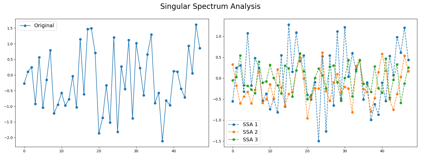
# Author: Johann Faouzi # License: BSD-3-Clause import numpy as np import matplotlib.pyplot as plt from pyts.decomposition import SingularSpectrumAnalysis # Parameters n_samples, n_timestamps = 100, 48 # Toy dataset rng = np.random.RandomState(41) X = rng.randn(n_samples, n_timestamps) # We decompose the time series into three subseries window_size = 15 groups = [np.arange(i, i + 5) for i in range(0, 11, 5)] # Singular Spectrum Analysis ssa = SingularSpectrumAnalysis(window_size=15, groups=groups) X_ssa = ssa.fit_transform(X) # Show the results for the first time series and its subseries plt.figure(figsize=(16, 6)) ax1 = plt.subplot(121) ax1.plot(X[0], 'o-', label='Original') ax1.legend(loc='best', fontsize=14) ax2 = plt.subplot(122) for i in range(len(groups)): ax2.plot(X_ssa[0, i], 'o--', label='SSA '.format(i + 1)) ax2.legend(loc='best', fontsize=14) plt.suptitle('Singular Spectrum Analysis', fontsize=20) plt.tight_layout() plt.subplots_adjust(top=0.88) plt.show() # The first subseries consists of the trend of the original time series. # The second and third subseries consist of noise. 

Total running time of the script: ( 0 minutes 3.365 seconds)

Источник