Python seaborn heatmap size

seaborn.heatmap#

seaborn. heatmap ( data , * , vmin = None , vmax = None , cmap = None , center = None , robust = False , annot = None , fmt = ‘.2g’ , annot_kws = None , linewidths = 0 , linecolor = ‘white’ , cbar = True , cbar_kws = None , cbar_ax = None , square = False , xticklabels = ‘auto’ , yticklabels = ‘auto’ , mask = None , ax = None , ** kwargs ) #

Plot rectangular data as a color-encoded matrix.

This is an Axes-level function and will draw the heatmap into the currently-active Axes if none is provided to the ax argument. Part of this Axes space will be taken and used to plot a colormap, unless cbar is False or a separate Axes is provided to cbar_ax .

Parameters : data rectangular dataset

2D dataset that can be coerced into an ndarray. If a Pandas DataFrame is provided, the index/column information will be used to label the columns and rows.

vmin, vmax floats, optional

Values to anchor the colormap, otherwise they are inferred from the data and other keyword arguments.

cmap matplotlib colormap name or object, or list of colors, optional

The mapping from data values to color space. If not provided, the default will depend on whether center is set.

center float, optional

The value at which to center the colormap when plotting divergent data. Using this parameter will change the default cmap if none is specified.

robust bool, optional

If True and vmin or vmax are absent, the colormap range is computed with robust quantiles instead of the extreme values.

annot bool or rectangular dataset, optional

If True, write the data value in each cell. If an array-like with the same shape as data , then use this to annotate the heatmap instead of the data. Note that DataFrames will match on position, not index.

fmt str, optional

String formatting code to use when adding annotations.

annot_kws dict of key, value mappings, optional

Keyword arguments for matplotlib.axes.Axes.text() when annot is True.

linewidths float, optional

Width of the lines that will divide each cell.

linecolor color, optional

Color of the lines that will divide each cell.

cbar bool, optional

Whether to draw a colorbar.

cbar_kws dict of key, value mappings, optional

cbar_ax matplotlib Axes, optional

Axes in which to draw the colorbar, otherwise take space from the main Axes.

square bool, optional

If True, set the Axes aspect to “equal” so each cell will be square-shaped.

xticklabels, yticklabels “auto”, bool, list-like, or int, optional

If True, plot the column names of the dataframe. If False, don’t plot the column names. If list-like, plot these alternate labels as the xticklabels. If an integer, use the column names but plot only every n label. If “auto”, try to densely plot non-overlapping labels.

mask bool array or DataFrame, optional

If passed, data will not be shown in cells where mask is True. Cells with missing values are automatically masked.

ax matplotlib Axes, optional

Axes in which to draw the plot, otherwise use the currently-active Axes.

kwargs other keyword arguments

All other keyword arguments are passed to matplotlib.axes.Axes.pcolormesh() .

Returns : ax matplotlib Axes

Axes object with the heatmap.

Plot a matrix using hierarchical clustering to arrange the rows and columns.

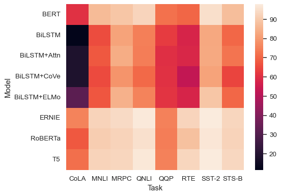
Pass a DataFrame to plot with indices as row/column labels:

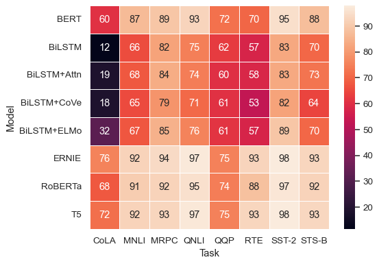
glue = sns.load_dataset("glue").pivot("Model", "Task", "Score") sns.heatmap(glue) 

/var/folders/qk/cdrdfhfn5g554pnb30pp4ylr0000gn/T/ipykernel_77613/2862412127.py:1: FutureWarning: In a future version of pandas all arguments of DataFrame.pivot will be keyword-only. glue = sns.load_dataset("glue").pivot("Model", "Task", "Score") 

Use annot to represent the cell values with text:

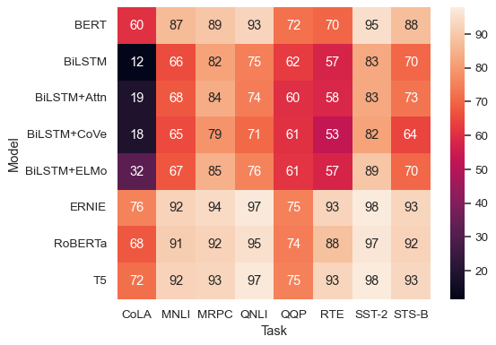
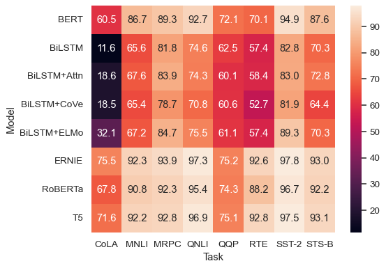
Control the annotations with a formatting string:

sns.heatmap(glue, annot=True, fmt=".1f") 

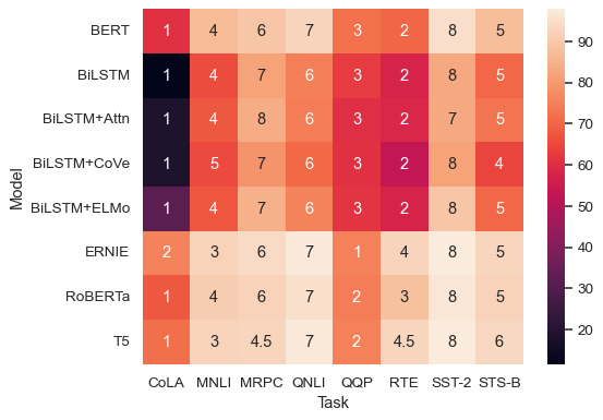
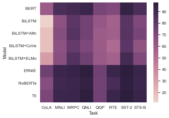
Use a separate dataframe for the annotations:

sns.heatmap(glue, annot=glue.rank(axis="columns")) 

sns.heatmap(glue, annot=True, linewidth=.5) 

Select a different colormap by name:

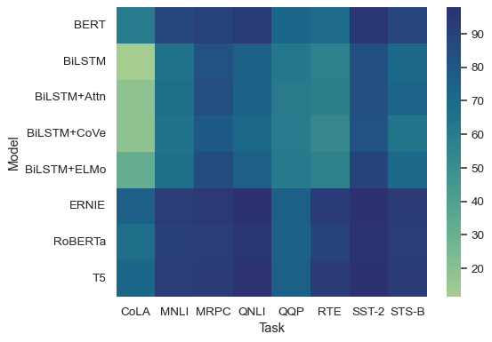
Or pass a colormap object:

sns.heatmap(glue, cmap=sns.cubehelix_palette(as_cmap=True)) 

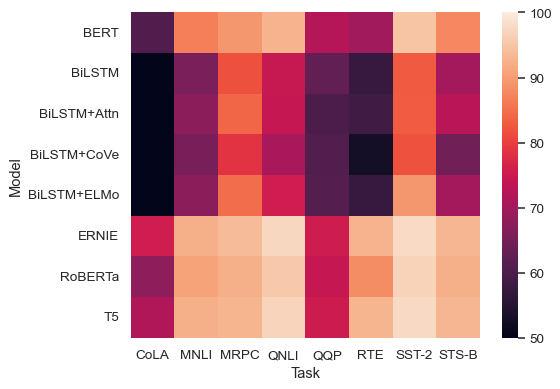
Set the colormap norm (data values corresponding to minimum and maximum points):

sns.heatmap(glue, vmin=50, vmax=100) 

Use methods on the matplotlib.axes.Axes object to tweak the plot:

ax = sns.heatmap(glue, annot=True) ax.set(xlabel="", ylabel="") ax.xaxis.tick_top() 

Источник

Как настроить размер тепловых карт в Seaborn

Вы можете использовать аргумент figsize , чтобы указать размер (в дюймах) тепловой карты моря :

#specify size of heatmap fig, ax = plt.subplots(figsize=(15, 5)) #create seaborn heatmap sns.heatmap(df) 

В следующем примере показано, как использовать этот синтаксис на практике.

Пример: настройка размера тепловых карт в Seaborn

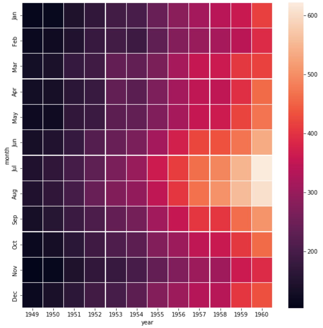
В этом примере мы будем использовать набор данных о морских перевозках под названием Flights, который содержит количество авиапассажиров, которые летали каждый месяц с 1949 по 1960 год:

import matplotlib.pyplot as plt import seaborn as sns #load "flights" dataset data = sns.load_dataset("flights") data = data.pivot(" month", " year", " passengers ") #view first five rows of dataset print(data.head()) year 1949 1950 1951 1952 1953 1954 1955 1956 1957 1958 1959 1960 month Jan 112 115 145 171 196 204 242 284 315 340 360 417 Feb 118 126 150 180 196 188 233 277 301 318 342 391 Mar 132 141 178 193 236 235 267 317 356 362 406 419 Apr 129 135 163 181 235 227 269 313 348 348 396 461 May 121 125 172 183 229 234 270 318 355 363 420 472 

Далее мы создадим тепловую карту, используя размеры figsize 10 на 10:

#specify size of heatmap fig, ax = plt.subplots(figsize=(10, 10)) #create heatmap sns.heatmap(data, linewidths= .3 ) 

Обратите внимание, что тепловая карта имеет одинаковые размеры по высоте и ширине.

Мы можем сделать тепловую карту более узкой, уменьшив первый аргумент в figsize :

#specify size of heatmap fig, ax = plt.subplots(figsize=(5, 10)) #create heatmap sns.heatmap(data, linewidths= .3 )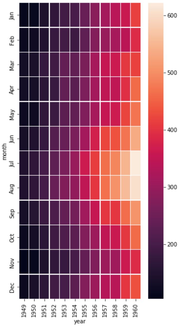 

Или мы могли бы сделать тепловую карту более широкой, уменьшив второй аргумент в figsize :

#specify size of heatmap fig, ax = plt.subplots(figsize=(10, 5)) #create heatmap sns.heatmap(data, linewidths= .3 )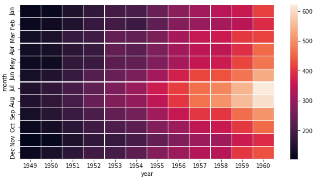 

Не стесняйтесь изменять значения в figsize , чтобы изменить размеры тепловой карты.

Дополнительные ресурсы

В следующих руководствах объясняется, как выполнять другие распространенные операции в Seaborn:

Источник

Seaborn Heatmap Size

To represent the data in a statistical graphical form, the “seaborn” Python package can be used that is built on the “matplotlib” library. It offers multiple features, and the “heatmap” is one of them that uses a color palette to depict variations in linked data. In the Seaborn module, the “sns.heatmap()” method is used for making heatmap charts.

What is Seaborn Heatmap Size in Python?

In Python, the seaborn heatmap size is utilized for the graphical representation of the matrix. It plots the graph matrix and uses the different shades of color for different types of values.

Let’s have a look at the provided examples for a better understanding!

Example 1: How to Set the Size of Seaborn Heatmap Using the “plt.set()” Function in Python?

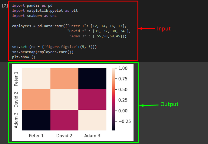
To set the size of the heatmap, the “plt.set()” method can be used along with the “rc” parameter and its value. To do so, first, import the Python’s required libraries, such as “matplotlib”, “pandas”, and “seaborn” libraries:

Then, use the “DataFrame()” method to create a new data frame named “employees” and add the values:

employees = pd. DataFrame ( { «Peter 1» : [ 12 , 14 , 16 , 17 ] ,
«David 2» : [ 31 , 32 , 38 , 34 ] ,
«Adam 3» : [ 55 , 58 , 59 , 45 ] } )

Now, call the “set()” method to adjust the size of the plot and pass the “rc” parameter along with its values according to your desire. After that, apply the “sns.heatmap()” function and use the “corr()” method to retrieve the correlation of each column in a specified data frame. Lastly, to display the resultant plot, use the “show()” method:

sns. set ( rc = { ‘figure.figsize’ : ( 5 , 3 ) } )
sns. heatmap ( employees. corr ( ) )
plt. show ( )

Output

Example 2: How to Set the Size of Seaborn Heatmap Using the “plt.figure()” Function in Python?

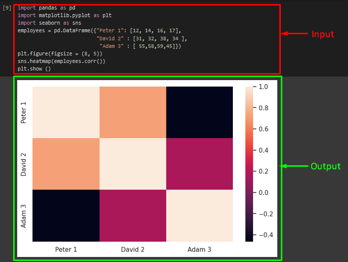
The “plt.figure()” function can be used to set the size of the seaborn heatmap. To do so, apply the “plt.figure()” method and pass the “figsize” parameter with the x-axis and y-axis sizes. Then, call the “sns.heatmap()” function and pass the data frame name as an argument along with the “corr()” method. To show the updated plot, invoke the “plt.show()” method:

As you can see, the size of the seaborn heatmap has been increased successfully:

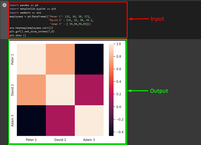
Example 3: How to Set the Size of Seaborn Heatmap Using the “plt.gcf()” Function in Python?

The “plt.gcf()” function is primarily utilized for getting the current figure. If it is used along with the “set_size_inches()” method, then it will resize the seaborn heatmap. For that particular purpose, apply the “plt.gcf().set_size_inches()” method with the height and width values. For visualization, call the “plt.show()” method:

That’s all! We have provided the details about the seaborn heatmap size in Python.

Conclusion

To resize the Seaborn heatmap in Python, the “plt.set()”, “plt.figure()”, and “plt.gcf” methods are used. The “plt.set()” method can be used along with the “rc” parameter and its value. The “plt.figure()” method takes the “figsize” parameter with the x-axis and y-axis sizes. The “plt.gcf()” method is used with the “set_size_inches()” method to set the height and width of the seaborn heatmap. This article illustrated the ways to resize the seaborn heatmap in Python.

About the author

Maria Naz

I hold a master’s degree in computer science. I am passionate about my work, exploring new technologies, learning programming languages, and I love to share my knowledge with the world.

Источник