Random forest classifier from scratch in Python
I recently learnt about Random Forest Classifiers/Regressors. It is a supervised machine learning technique that performs well on interpolation problems. It was formally introduced in 2001 by Leo Breiman. They are much easier to train and much smaller than the more modern, but more powerful, neural networks. They are often included in major machine learning software and libraries, including R and Scikit-learn.
There are many article describing the theory behind random forests. See for example 1 or 2. By far the best and most detailed explanation I have seen is given by Jeremy Howard in his FastAI course. A few sources describe how to implement them from scratch, such as 3 or 4.
My aim here is to describe my own implementation of a random forest from scratch for teaching purposes. It is assumed the reader is already familiar with the theory. I hope this post will clarify in-depth questions. The first version was based on the code in the FastAI course, but I have made it more advanced. The full code can be accessed at my Github repository. The version presented here is slightly simpler and more compact.
Scikit-learn’s RandomForestClassifier is far superior to mine. It is written in several thousand lines of code; mine was written in just 270. The main advantages of it are:
- it is much faster (by more than 100x) because it is written in Cython, utilises multiple cores to parallelise jobs and also because of more advanced coding optimisation algorithms.
- it has more options and features for the user.
- it does more data validation and input checking.
Having been inspired by Jeremy Howard’s teaching methods, I will present this post in a top-down fashion. First I’ll introduce two datasets and show how the random forest classifier can be used on them. Next, I’ll explain the top level RandomForestClassifier class, then the DecisionTree class it is composed of, and finally the BinaryTree class that that is composed of. All code is also explained top-down.
Practice Data Sets
The Iris flower dataset
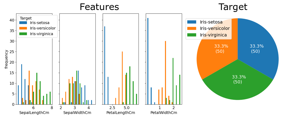
The Iris flower dataset is commonly used for beginner machine learning problems. The full dataset can be found on Kaggle at www.kaggle.com/arshid/iris-flower-dataset. It consists of 150 entries for 3 types of iris plants, and 4 features: sepal length and width, and petal length and width. 1
The variable distributions are as follows:
Based on these, a simple baseline model can be developed:
- If PetalLength < 2.5cm, class is Setosa.
- Else determine scores score1 and score2 as follows:
- score1: add 1 for each of the following that is true:
- 2.5cm < PetalLength ≤ 5.0cm
- 1.0cm≤ PetalWidth ≤ 1.8cm
- score2: add 1 for each of the following that is true:
- 7.0cm≤ SepalLength
- 3.5cm≤ SepalWidth
- 5.0cm≤ PetalLength
- 1.7cm < PetalWidth
- score1: add 1 for each of the following that is true:
- If score1 > score2, classify as Veriscolor. If score1 < score2, classify as Virginica. If score1 = score2, leave unknown, or classify at random.
This simple strategy guarantees that 140 samples, which is 93.3% of the samples, will be correctly classified.
I used my code to make a random forest classifier with the following parameters:
forest = RandomForestClassifier(n_trees=10, bootstrap=True, max_features=2, min_samples_leaf=3)
I randomly split the data into 120 training samples and 30 test samples. The forest took 0.23 seconds to train. It had trees with depths in the range of 3 to 7, and 65 leaves in total. It misclassified one sample in the training and test set each, for an accuracy of 99.2% and 96.7% respectively. This is a clear improvement on the baseline.
This is a simple flattened representation of one of the trees. Each successive dash represents a level lower in the tree, and left children come before right:
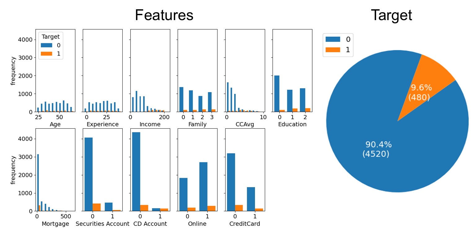
The Pearson correlation coefficients between the features and the target variables are:
| Feature | Correlation | |
|---|---|---|
| 1 | Income | 0.5025 |
| 2 | CCAvg | 0.3669 |
| 3 | CD Account | 0.3164 |
| 4 | Mortgage | 0.1421 |
| 5 | Education | 0.1367 |
| 6 | Family | 0.0614 |
| 7 | Securities Account | 0.0220 |
| 8 | Experience | -0.0074 |
| 9 | Age | -0.0077 |
| 10 | Online | 0.0063 |
| 11 | CreditCard | 0.0028 |
For the baseline model, we could always predict a 0, and claim an accuracy of 90.4%. But this has an F1 score of 0. 2 A better baseline is simply to have: 1 if Income > 100 else 0. This has an accuracy of 83.52% and a F1 score of 0.516 over the whole dataset.
I used my code to make a random forest classifier with the following parameters:
forest = RandomForestClassifier(n_trees=20, bootstrap=True, max_features=3, min_samples_leaf=3)
I randomly split the data into 4000 training samples and 1000 test samples and trained the forest on it. The forest took about 10 seconds to train. The trees range in depth from 11 to 17, with 51 to 145 leaves. The total number of leaves is 1609. The training accuracy is 99.60% and the test accuracy is 98.70%. The F1 score for the test set is 0.926. This is a large improvement on the baseline, especially for the F1 score.
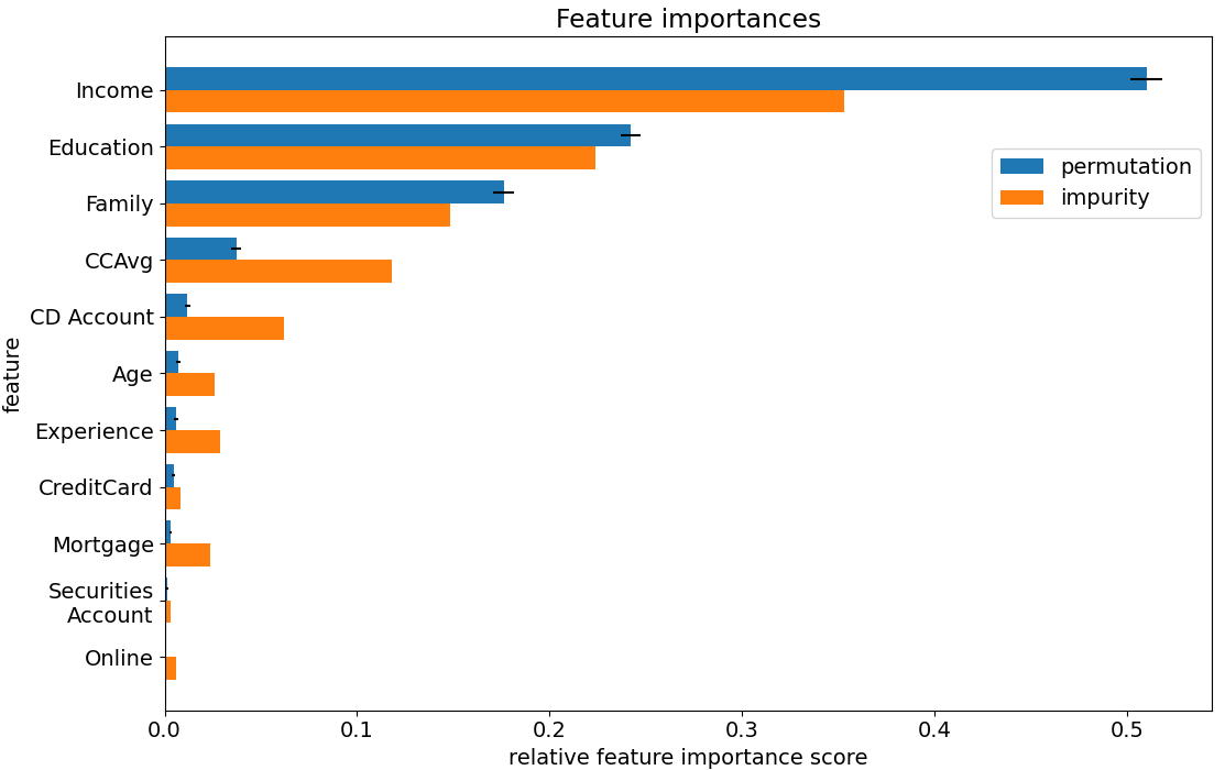
We can inspect the random forest and calculate a feature importance for each feature. The following graph is a comparison between two types of (normalised) feature importances. The orange bars are based on how much that feature contributes to decreasing the impurity levels in the tree. The blue bars are based on randomly scrambling that feature column, and recording how much this decreases the overall accuracy of the model. More detail on these calculations will be given later.
Code
RandomForestClassifier
The first step is create the RandomForestClassifier . Initialising an instance of the class only sets the internal parameters and does not fit the data, as with the equivalent Scikit-learn class. I’ve included the most important parameters from Scikit-learn, and added one of my own, sample_size . 3 This parameter sets the sample size used to make each tree. If bootstrap=False , it will randomly select a subset of unique samples for the training dataset. If bootstrap=True , it will randomly draw samples with replacement from the dataset, which will most likely result in duplicate samples.
The most direct way to code a binary tree is to do so as a linked list. Each node is an object with pointers to its children. This was the method originally used in the FastAI course. The method that Scikit-learn uses, and that I chose to use, is to encode it as a set of two parallel lists. The image above shows an example of this representation. The index is the node ID, and the values in the left and right array are the node IDs (indexes) for that node’s children. If the value is -1, it means this node has no children and is a leaf. This method is more compact than the linked list, and has an O(1) look-up time for children given a node ID.
This is the smallest and simplest class, and so I will present the entire code here without further explanation:
class BinaryTree(): def __init__(self): self.children_left = [] self.children_right = [] @property def n_leaves(self): return self.children_left.count(-1) def add_node(self): self.children_left.append(-1) self.children_right.append(-1) def set_left_child(self, node_id: int, child_id: int): self.children_left[node_id] = child_id def set_right_child(self, node_id: int, child_id: int): self.children_right[node_id] = child_id def get_children(self, node_id: int) -> Tuple[int]: return self.children_left[node_id], self.children_right[node_id] def is_leaf(self, node_id: int) -> bool: return self.children_left[node_id] == self.children_right[node_id] #==-1Conclusion
I hope you enjoyed this post, and that it clarified the inner workings of a random forest. If you would like to know more, I again recommend Jeremy Howard’s FastAI course. He explains the rational behind random forests, more on tree interpretation and more on the limitations of random forests.
What did you think of the top-down approach? I think it works very well.
In the future, I would like to investigate more advanced versions of tree ensembles, in particular gradient boosting techniques like CatBoost.
- Don’t know what a sepal is? I didn’t either. It’s the outer part of the flower that encloses the bud. Basically it’s a leaf that looks like a petal. ↩
- The F1 score balances recall (fraction of true positives predicted) with precision (fraction of correct positives). Guessing all true would have high recall but low precision. It is better to have both. $F1 =\frac>+\frac>>$ ↩
- It is annoying that the Scikit-learn module does not include this parameter. There are ways around it. For example the FastAI package edits the Scikit-learn code with set_rf_samples() . Or you could sample data yourself and train a tree one at a time using the warm_start=True parameter. But these are hacks for what I think could have been a simple input parameter. ↩
- Let the sample size be k and the total number of samples be n. Then the probability that there is at least one version of any particular sample is: \(\begin P(\text) &= P(\text) + P(\text) + . + P(k \text< versions>) \\ &= 1 — P(\text) \\ &= 1 — \left (\frac\right)^k \\\undersetP(\text) &= 1 — e^\\\end\).
For n=k, $P(\text)\rightarrow 1-e^ = 0.63212…$ ↩ - Another way would probably be to determine the distribution of values e.g. linear, exponential, categorical. Then use this information to create a good feature range. ↩
Adapted from Clean Blog theme by Start Bootstrap
Copyright © Lior Sinai 2023
Random Forest Classifier in Python Sklearn with Example
In this article, we will see the tutorial for implementing random forest classifier using the Sklearn (a.k.a Scikit Learn) library of Python. We will first cover an overview of what is random forest and how it works and then implement an end-to-end project with a dataset to show an example of Sklean random forest with RandomForestClassifier() function.
What is Random Forest
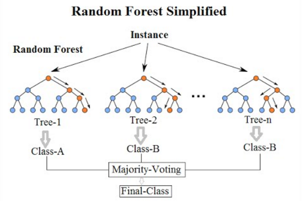
Random forest is a supervised machine learning algorithm used to solve classification as well as regression problems. It is a type of ensemble learning technique in which multiple decision trees are created from the training dataset and the majority output from them is considered as the final output.
Random forest is a very popular technique due to its simplicity and ability to produce robust results.
How Random Forest Works
Random Forest works on the Bootstrap Aggregation (Bagging) technique of Ensemble learning –
i) Here, first of all, multiple training data is created by sampling data from the training set which is known as bootstrapping or bagging.
For example, if we have a data set (a,b,c,d,e,f,g,h,i,j) then the following training set can be obtained with bootstrap –
You may notice here that the same data can appear multiple times across the training sets because we are doing random sampling with replacement.
ii) The leftover training data that has not been added in the bootstrapped data can be used to find the random forest accuracy. This is called the out-of-bag-datasets.
iii) Next, multiple decision trees are trained on each of these datasets. Instead of taking all features, we can add more variation by randomly selecting some features of the dataset for each of the decision trees.
iv) The output of each decision tree is aggregated to produce the final output. For classification, the aggregation is done by choosing the majority vote from the decision trees for classification. In the case of regression, the aggregation can be done by averaging the outputs from all the decision trees.
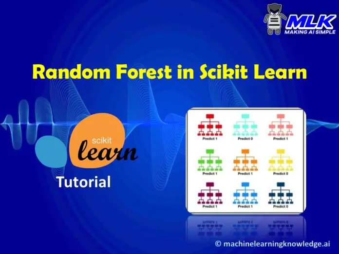
e.g. if 9 decision trees are created for the random forest classifier, and 6 of them classify the outputs as class 1 and the remaining 3 classify output as class 0, then the final classification will be chosen as class 1, based on the maximum vote it got.
