Python полиномиальная линия тренда

sklearn.preprocessing .PolynomialFeatures¶

Generate a new feature matrix consisting of all polynomial combinations of the features with degree less than or equal to the specified degree. For example, if an input sample is two dimensional and of the form [a, b], the degree-2 polynomial features are [1, a, b, a^2, ab, b^2].

Parameters : degree int or tuple (min_degree, max_degree), default=2

If a single int is given, it specifies the maximal degree of the polynomial features. If a tuple (min_degree, max_degree) is passed, then min_degree is the minimum and max_degree is the maximum polynomial degree of the generated features. Note that min_degree=0 and min_degree=1 are equivalent as outputting the degree zero term is determined by include_bias .

interaction_only bool, default=False

If True , only interaction features are produced: features that are products of at most degree distinct input features, i.e. terms with power of 2 or higher of the same input feature are excluded:

If True (default), then include a bias column, the feature in which all polynomial powers are zero (i.e. a column of ones — acts as an intercept term in a linear model).

order , default=’C’

Order of output array in the dense case. ‘F’ order is faster to compute, but may slow down subsequent estimators.

Exponent for each of the inputs in the output.

n_features_in_ int

Number of features seen during fit .

Names of features seen during fit . Defined only when X has feature names that are all strings.

The total number of polynomial output features. The number of output features is computed by iterating over all suitably sized combinations of input features.

Transformer that generates univariate B-spline bases for features.

Be aware that the number of features in the output array scales polynomially in the number of features of the input array, and exponentially in the degree. High degrees can cause overfitting.

>>> import numpy as np >>> from sklearn.preprocessing import PolynomialFeatures >>> X = np.arange(6).reshape(3, 2) >>> X array([[0, 1], [2, 3], [4, 5]]) >>> poly = PolynomialFeatures(2) >>> poly.fit_transform(X) array([[ 1., 0., 1., 0., 0., 1.], [ 1., 2., 3., 4., 6., 9.], [ 1., 4., 5., 16., 20., 25.]]) >>> poly = PolynomialFeatures(interaction_only=True) >>> poly.fit_transform(X) array([[ 1., 0., 1., 0.], [ 1., 2., 3., 6.], [ 1., 4., 5., 20.]]) 

Compute number of output features.

Fit to data, then transform it.

Get output feature names for transformation.

Get metadata routing of this object.

Get parameters for this estimator.

Set the parameters of this estimator.

Transform data to polynomial features.

Compute number of output features.

Parameters : X of shape (n_samples, n_features)

Not used, present here for API consistency by convention.

Returns : self object

Fit to data, then transform it.

Fits transformer to X and y with optional parameters fit_params and returns a transformed version of X .

Parameters : X array-like of shape (n_samples, n_features)

y array-like of shape (n_samples,) or (n_samples, n_outputs), default=None

Target values (None for unsupervised transformations).

**fit_params dict

Additional fit parameters.

Returns : X_new ndarray array of shape (n_samples, n_features_new)

get_feature_names_out ( input_features = None ) [source] ¶

Get output feature names for transformation.

Parameters : input_features array-like of str or None, default=None

• If input_features is None , then feature_names_in_ is used as feature names in. If feature_names_in_ is not defined, then the following input feature names are generated: [«x0», «x1», . «x(n_features_in_ — 1)»] .
• If input_features is an array-like, then input_features must match feature_names_in_ if feature_names_in_ is defined.

Transformed feature names.

Get metadata routing of this object.

Please check User Guide on how the routing mechanism works.

Returns : routing MetadataRequest

A MetadataRequest encapsulating routing information.

Get parameters for this estimator.

Parameters : deep bool, default=True

If True, will return the parameters for this estimator and contained subobjects that are estimators.

Returns : params dict

Parameter names mapped to their values.

Exponent for each of the inputs in the output.

See Introducing the set_output API for an example on how to use the API.

Parameters : transform , default=None

Configure output of transform and fit_transform .

• «default» : Default output format of a transformer
• «pandas» : DataFrame output
• None : Transform configuration is unchanged

Set the parameters of this estimator.

The method works on simple estimators as well as on nested objects (such as Pipeline ). The latter have parameters of the form __ so that it’s possible to update each component of a nested object.

Parameters : **params dict

Returns : self estimator instance

Transform data to polynomial features.

Parameters : X of shape (n_samples, n_features)

The data to transform, row by row.

Prefer CSR over CSC for sparse input (for speed), but CSC is required if the degree is 4 or higher. If the degree is less than 4 and the input format is CSC, it will be converted to CSR, have its polynomial features generated, then converted back to CSC.

If the degree is 2 or 3, the method described in “Leveraging Sparsity to Speed Up Polynomial Feature Expansions of CSR Matrices Using K-Simplex Numbers” by Andrew Nystrom and John Hughes is used, which is much faster than the method used on CSC input. For this reason, a CSC input will be converted to CSR, and the output will be converted back to CSC prior to being returned, hence the preference of CSR.

Returns : XP of shape (n_samples, NP)

The matrix of features, where NP is the number of polynomial features generated from the combination of inputs. If a sparse matrix is provided, it will be converted into a sparse csr_matrix .

Источник

Как добавить линию тренда в Matplotlib (с примером)

Вы можете использовать следующий базовый синтаксис, чтобы добавить линию тренда на график в Matplotlib:

#create scatterplot plt.scatter (x, y) #calculate equation for trendline z = np.polyfit (x, y, 1) p = np.poly1d (z) #add trendline to plot plt.plot (x, p(x)) 

В следующих примерах показано, как использовать этот синтаксис на практике.

Пример 1: создание линейной линии тренда в Matplotlib

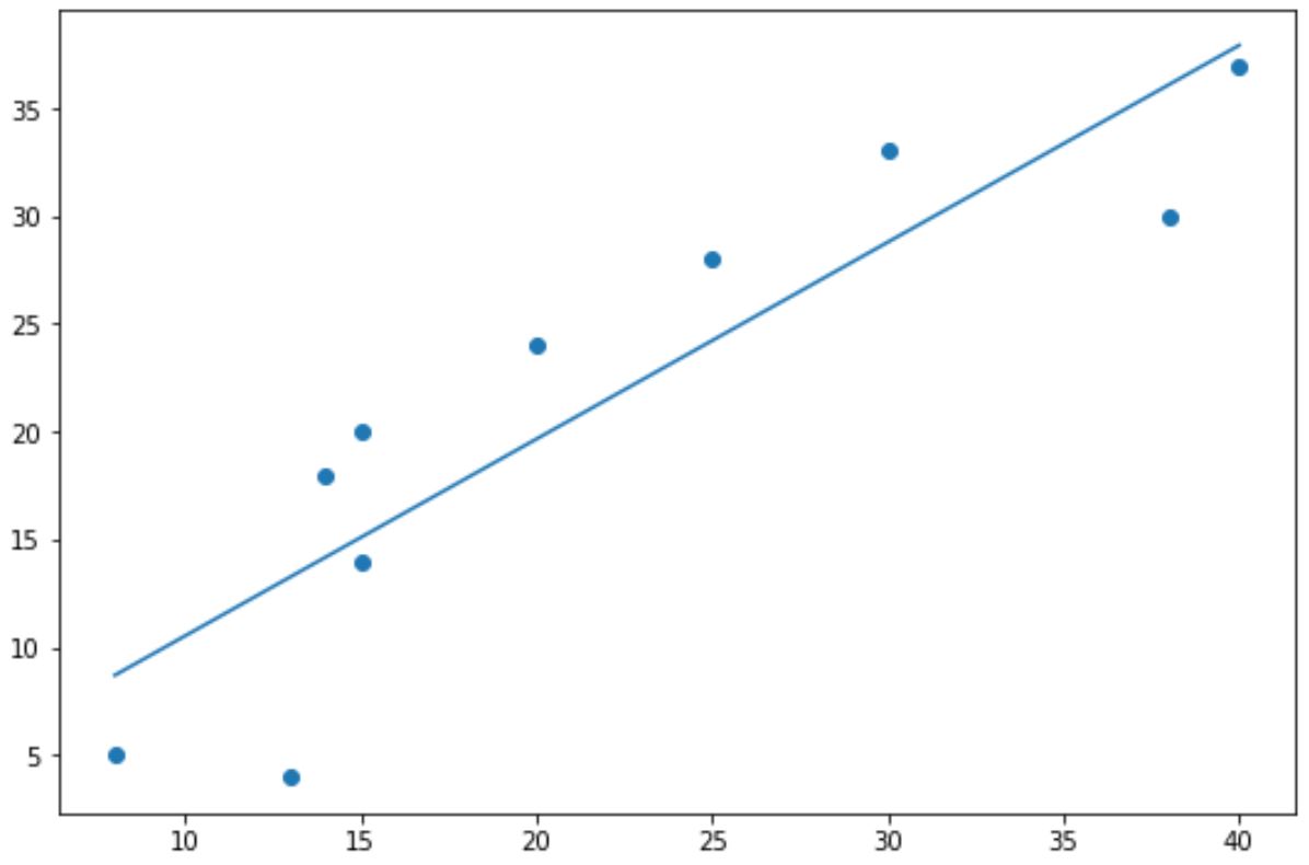
В следующем коде показано, как создать базовую линию тренда для диаграммы рассеяния в Matplotlib:

import numpy as np import matplotlib.pyplot as plt #define data x = np.array([8, 13, 14, 15, 15, 20, 25, 30, 38, 40]) y = np.array([5, 4, 18, 14, 20, 24, 28, 33, 30, 37]) #create scatterplot plt.scatter (x, y) #calculate equation for trendline z = np.polyfit (x, y, 1 ) p = np.poly1d (z) #add trendline to plot plt.plot (x, p(x)) 

Синие точки представляют точки данных, а прямая синяя линия представляет собой линейную линию тренда.

Обратите внимание, что вы также можете использовать аргументы color , linewidth и linestyle для изменения внешнего вида линии тренда:

#add custom trendline to plot plt.plot (x, p(x), color=" purple", linewidth= 3 , linestyle=" -- ")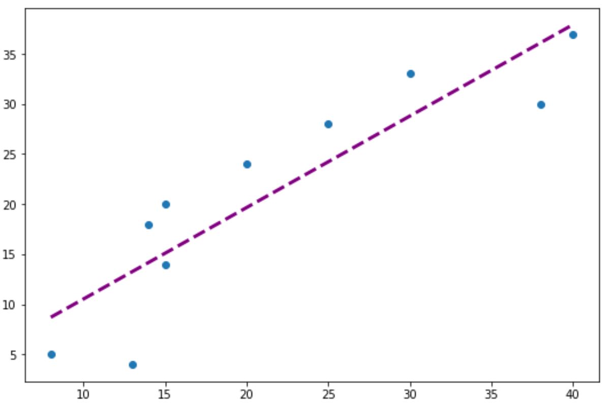 

Пример 2: создание полиномиальной линии тренда в Matplotlib

Чтобы создать полиномиальную линию тренда, просто измените значение в функции np.polyfit() .

Например, мы могли бы использовать значение 2 для создания квадратичной линии тренда:

import numpy as np import matplotlib.pyplot as plt #define data x = np.array([8, 13, 14, 15, 15, 20, 25, 30, 38, 40]) y = np.array([5, 4, 18, 14, 20, 24, 28, 33, 30, 37]) #create scatterplot plt.scatter (x, y) #calculate equation for quadratic trendline z = np.polyfit (x, y, 2 ) p = np.poly1d (z) #add trendline to plot plt.plot (x, p(x))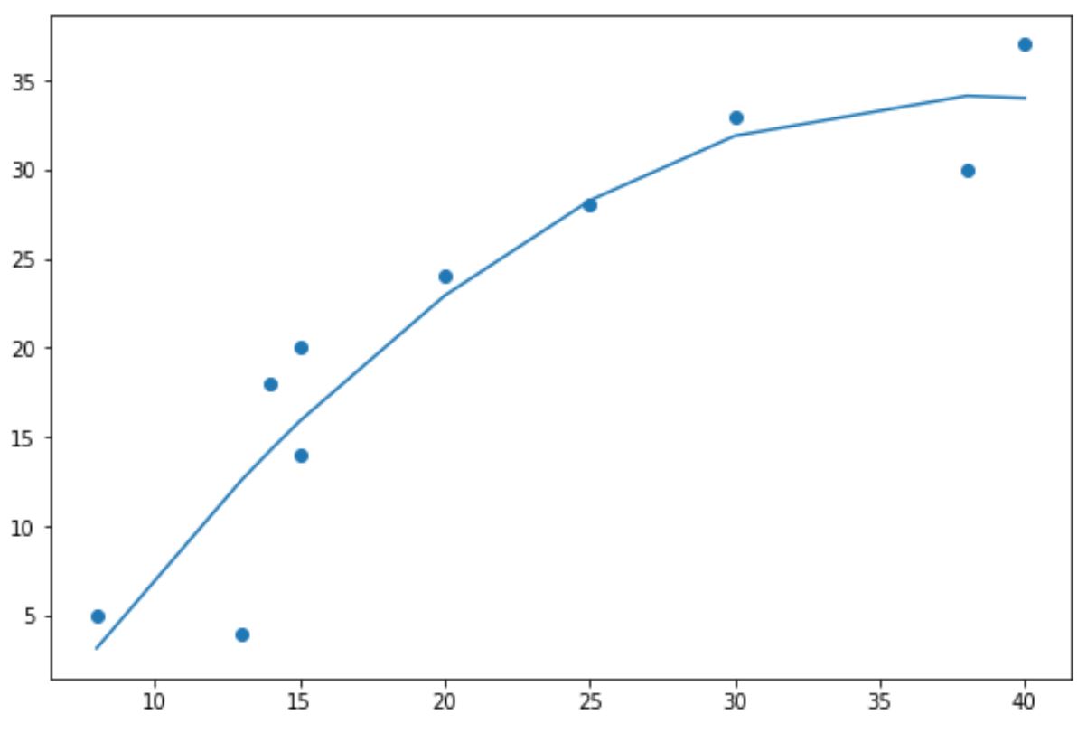 

Обратите внимание, что линия тренда теперь изогнута, а не прямая.

Эта полиномиальная линия тренда особенно полезна, когда ваши данные демонстрируют нелинейный шаблон, а прямая линия плохо отражает тренд в данных.

Дополнительные ресурсы

В следующих руководствах объясняется, как выполнять другие распространенные функции в Matplotlib:

Источник

Как выполнить полиномиальную регрессию в Python

Регрессионный анализ используется для количественной оценки взаимосвязи между одной или несколькими независимыми переменными и переменной отклика.

Наиболее распространенным типом регрессионного анализа является простая линейная регрессия , которая используется, когда переменная-предиктор и переменная-отклик имеют линейную связь.

Однако иногда связь между переменной-предиктором и переменной-ответом нелинейна.

Например, истинное отношение может быть квадратичным:

Или он может быть кубическим:

В этих случаях имеет смысл использовать полиномиальную регрессию , которая может учитывать нелинейную связь между переменными.

В этом руководстве объясняется, как выполнить полиномиальную регрессию в Python.

Пример: полиномиальная регрессия в Python

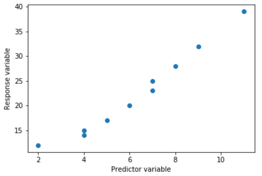
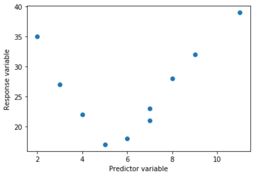
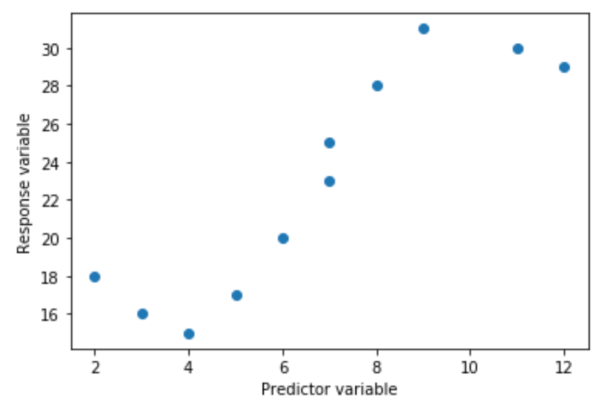
Предположим, у нас есть следующая предикторная переменная (x) и переменная ответа (y) в Python:

x = [2, 3, 4, 5, 6, 7, 7, 8, 9, 11, 12] y = [18, 16, 15, 17, 20, 23, 25, 28, 31, 30, 29] 

Если мы создадим простую диаграмму рассеяния этих данных, мы увидим, что связь между x и y явно нелинейна:

import matplotlib.pyplot as plt #create scatterplot plt.scatter(x, y)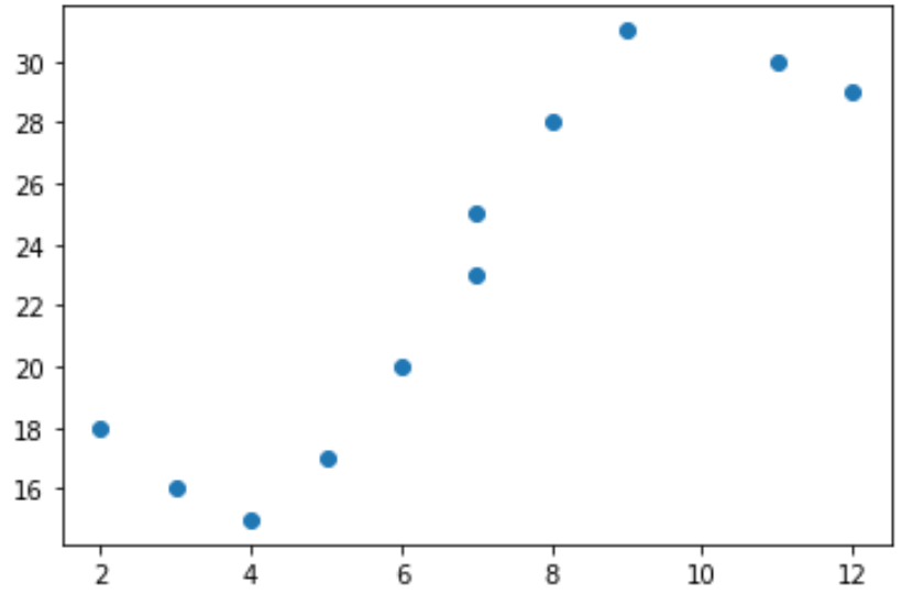 

Таким образом, не имеет смысла подгонять к этим данным модель линейной регрессии. Вместо этого мы можем попытаться подобрать модель полиномиальной регрессии со степенью 3, используя функцию numpy.polyfit() :

import numpy as np #polynomial fit with degree = 3 model = np.poly1d(np.polyfit(x, y, 3)) #add fitted polynomial line to scatterplot polyline = np.linspace(1, 12, 50) plt.scatter(x, y) plt.plot(polyline, model(polyline)) plt.show()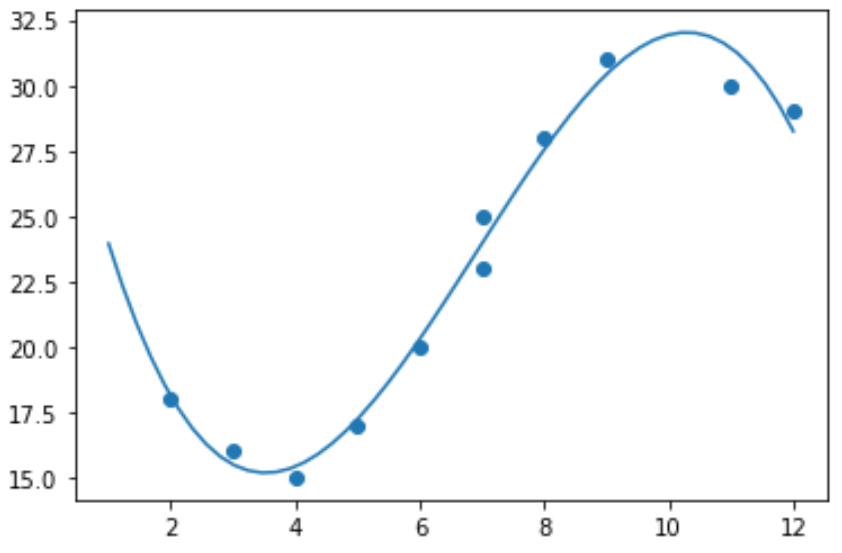 

Мы можем получить подобранное уравнение полиномиальной регрессии, напечатав коэффициенты модели:

print(model) poly1d([ -0.10889554, 2.25592957, -11.83877127, 33.62640038]) 

Подходящее уравнение полиномиальной регрессии:

у = -0,109 х 3 + 2,256 х 2 – 11,839 х + 33,626

Это уравнение можно использовать для нахождения ожидаемого значения переменной отклика на основе заданного значения объясняющей переменной. Например, предположим, что x = 4. Ожидаемое значение переменной ответа y будет следующим:

у = -0,109(4) 3 + 2,256(4) 2 – 11,839(4) + 33,626= 15,39 .

Мы также можем написать короткую функцию для получения R-квадрата модели, который представляет собой долю дисперсии переменной отклика, которая может быть объяснена переменными-предикторами.

#define function to calculate r-squared def polyfit(x, y, degree): results = <> coeffs = numpy.polyfit(x, y, degree) p = numpy.poly1d(coeffs) #calculate r-squared yhat = p(x) ybar = numpy.sum(y)/len(y) ssreg = numpy.sum((yhat-ybar)\*\*2) sstot = numpy.sum((y - ybar)\*\*2) results['r_squared'] = ssreg / sstot return results #find r-squared of polynomial model with degree = 3 polyfit(x, y, 3)

В этом примере R-квадрат модели равен 0,9841.Это означает, что 98,41% вариации переменной отклика можно объяснить предикторными переменными.

Источник