14 — Panel Data and Fixed Effects#
In the previous chapter, we explored a very simple Diff-in-Diff setup, where we had a treated and a control group (the city of POA and FLN, respectively) and only two periods, a pre-intervention and a post-intervention period. But what would happen if we had more periods? Or more groups? Turns out this setup is so common and powerful for causal inference that it gets its own name: panel data. A panel is when we have repeated observations of the same unit over multiple periods of time. This happens a lot in government policy evaluation, where we can track data on multiple cities or states over multiple years. But it is also incredibly common in the industry, where companies track user data over multiple weeks and months.
To understand how we can leverage such data structure, let’s first continue with our diff-in-diff example, where we wanted to estimate the impact of placing a billboard (treatment) in the city of Porto Alegre (POA). We want to see if that sort of offline marketing strategy can boost the usage of our investment products. Specifically, we want to know how much deposits in our investments account would increase if we placed billboards.
In the previous chapter, we’ve motivated the DiD estimator as an imputation strategy of what would have happened to Porto Alegre had we not placed the billboards in it. We said that the counterfactual outcome \(Y_0\) for Porto Alegre after the intervention (placing a billboard) could be inputted as the number of deposits in Porto Alegre before the intervention plus a growth factor. This growth factor was estimated in a control city, Florianopolis (FLN). Just so we can recap some notation, here is how we can estimate this counterfactual outcome
where \(t\) denotes time, \(D\) denotes the treatment (since \(t\) is taken), \(Y_D(t)\) denote the potential outcome for treatment \(D\) in period \(t\) (for example, \(Y_0(1)\) is the outcome under the control in period 1). Now, if we take that imputed potential outcome, we can recover the treatment effect for POA (ATT) as follows
In other words, the effect of placing a billboard in POA is the outcome we saw on POA after placing the billboard minus our estimate of what would have happened if we hadn’t placed the billboard. Also, recall that the power of DiD comes from the fact that estimating the mentioned counterfactual only requires that the growth deposits in POA matches the growth in deposits in FLW. This is the key parallel trends assumption. We should definitely spend some time on it because it is going to become very important later on.
Parallel Trends#
One way to see the parallel (or common) trends assumptions is as an independence assumption. If we recall from very early chapters, the independence assumption requires that the treatment assignment is independent from the potential outcomes:
This means we don’t give more treatment to units with higher outcome (which would cause upward bias in the effect estimation) or lower outcome (which would cause downward bias). In less abstract terms, back to our example, let’s say that your marketing manager decides to add billboards only to cities that already have very high deposits. That way, he or she can later boast that cities with billboards generate more deposties, so of course the marketing campaign was a success. Setting aside the moral discussion here, I think you can see that this violates the independence assumption: we are giving the treatment to cities with high \(Y_0\) . Also, remember that a natural extension of this assumption is the conditional independence assumption, which allows the potential outcomes to be dependent on the treatment at first, but independent once we condition on the confounders \(X\)
You know all of this already. But how exactly does this tie back to DiD and the parallel trends assumption? If the traditional independence assumption states that the treatment assignment can’t be related to the levels of potential outcomes, the parallel trends states that the treatment assignment can’t be related to the growth in potential outcomes over time. In fact, one way to write the parallel trends assumption is as follows
\( \big(Y_d(t) — Y_d(t-1) \big) \perp D \)
In less mathematical terms, this assumption is saying it is fine that we assign the treatment to units that have a higher or lower level of the outcome. What we can’t do is assign the treatment to units based on how the outcome is growing. In out billboard example, this means it is OK to place billboards only in cities with originally high deposits level. What we can’t do is place billboards only in cities where the deposits are growing the most. That makes a lot of sense if we remember that DiD is inputting the counterfactual growth in the treated unit with the growth in the control unit. If growth in the treated unit under the control is different than the growth in the control unit, then we are in trouble.
Controlling What you Cannot See#
Methods like propensity score, linear regression and matching are very good at controlling for confounding in non-random data, but they rely on a key assumption: conditional unconfoundedness
To put it in words, they require that all the confounders are known and measured, so that we can condition on them and make the treatment as good as random. One major issue with this is that sometimes we simply can’t measure a confounder. For instance, take a classical labor economics problem of figuring out the impact of marriage on men’s earnings. It’s a well known fact in economics that married men earn more than single men. However, it is not clear if this relationship is causal or not. It could be that more educated men are both more likely to marry and more likely to have a high earnings job, which would mean that education is a confounder of the effect of marriage on earnings. For this confounder, we could measure the education of the person in the study and run a regression controlling for that. But another confounder could be beauty. It could be that more handsome men are both more likely to get married and more likely to have a high paying job. Unfortunately, beauty is one of those characteristics like intelligence. It’s something we can’t measure very well.
This puts us in a difficult situation, because if we have unmeasured confounders, we have bias. One way to deal with this is with instrumental variables, as we’ve seen before. But coming up with good instruments it’s no easy task and requires a lot of creativity. Here, instead let’s take advantage of our panel data structure.
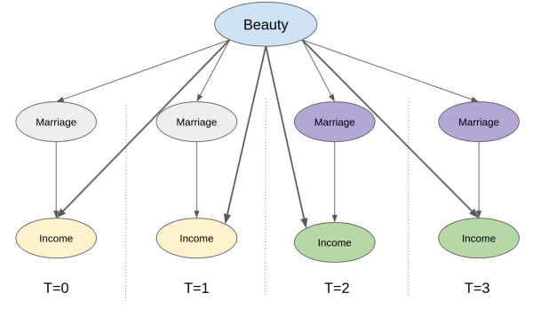
We’ve already seen how panel data allows us to replace the unconfoundedness assumption with the parallel trends assumption. But how exactly does this help with unmeasured confounders? First, let’s take a look at the causal graph which represents this setup where we have repeated observations across time. Here, we track the same observation across 4 time periods. Marriage (the treatment) and Income (the outcome) change over time. Specifically, marriage turns on (from 0 to 1) at period 3 and 4 and income increases in the same periods. Beauty, the unmeasured confounder, is the same across all periods (a bold statement, but reasonable if time is just a few years). So, how can we know that the reason income increases is because of marriage and not simply due to an increase in the beauty confounder? And, more importantly, how can we control that confounder we cannot see?
The trick is to see that, by zooming in a unit and tracking how it evolves over time, we are already controlling for anything that is fixed over time. That includes any time fixed unmeasured confounders. In the graph above, for instance, we can already know that the increase in income over time cannot be due to an increase in beauty, simply because beauty stays the same (it is time fixed after all). The bottom line is that even though we cannot control for beauty, since we can’t measure it, we can still use the panel structure so it is not a problem anymore.
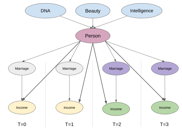
Another way of seeing this is to think about these time fixed confounders as attributes that are specific to each unit. This would be equivalent to adding an intermediary unit node to our causal graph. Now, notice how controlling for the unit itself already blocks the backdoor path between the outcome and any of the unobserved but time fixed confounders.
Think about it. We can’t measure attributes like beauty and intelligence, but we know that the person who has them is the same individual across time. The mechanics of actually doing this control is very simple. All we need to do is create dummy variables indicating that person and add that to a linear model. This is what we mean when we say we can control for the person itself: we are adding a variable (dummy in this case) that denotes that particular person. When estimating the effect of marriage on income with this person dummy in our model, regression finds the effect of marriage while keeping the person variable fixed. Adding this unit dummy is what we call a fixed effect model.
Fixed Effects#
To make matters more formal, let’s first take a look at the data that we have. Following our example, we will try to estimate the effect of marriage on income. Our data contains those 2 variables, married and lwage , on multiple individuals ( nr ) for multiple years. Notice that wage is in log form. In addition to this, we have other controls, like number of hours worked that year, years of education and so on.
data = wage_panel.load() data.head()
linearmodels.panel.model.PanelOLS
Dependent (left-hand-side) variable (time by entity).
Exogenous or right-hand-side variables (variable by time by entity).
Weights to use in estimation. Assumes residual variance is proportional to inverse of weight to that the residual time the weight should be homoskedastic.
Flag whether to include entity (fixed) effects in the model
Flag whether to include time effects in the model
Category codes to use for any effects that are not entity or time effects. Each variable is treated as an effect.
Flag indicating whether to drop singleton observation
Flag indicating whether to drop absorbed variables
Flag indicating whether to perform a rank check on the exogenous variables to ensure that the model is identified. Skipping this check can reduce the time required to validate a model specification. Results may be numerically unstable if this check is skipped and the matrix is not full rank.
Many models can be estimated. The most common included entity effects and can be described
where \(\alpha_i\) is included if entity_effects=True .
Time effect are also supported, which leads to a model of the form
where \(\gamma_i\) is included if time_effects=True .
Both effects can be simultaneously used,
Additionally , arbitrary effects can be specified using categorical variables.
If both entity_effect and time_effects are False , and no other effects are included, the model reduces to PooledOLS .
Model supports at most 2 effects. These can be entity-time, entity-other, time-other or 2 other.
fit (*[, use_lsdv, use_lsmr, low_memory, . ])
Estimate model parameters
Create a model from a formula
predict (params, *[, exog, data, eval_env, . ])
Predict values for additional data
Reformat cluster variables
Flag indicating whether entity effects are included
Formula used to construct the model
Flag indicating the model a constant or implicit constant
Locations of non-missing observations
Flag indicating whether other (generic) effects are included
Flag indicating whether time effects are included

