- Программа OpenCV Canny Edge Detection – распознавание границ объекта
- Синтаксис
- Параметры
- Пример 1
- Пример: обнаружение границ в реальном времени
- Python opencv cv2 canny
- Theory
- Canny Edge Detection in OpenCV
- Python opencv cv2 canny
- Theory
- Canny Edge Detection in OpenCV
- OpenCV Edge Detection in Python with cv2.Canny()
- Canny Edge Detection
- Edge Detection on Images with cv2.Canny()
Программа OpenCV Canny Edge Detection – распознавание границ объекта
Canny Edge Detection — это термин, обозначающий границу объекта на изображении. Мы узнаем о нем, используя технику обнаружения краев OpenCV Canny Edge Detection.
Синтаксис
Синтаксис функции обнаружения краев:
edges = cv2.Canny('/path/to/img', minVal, maxVal, apertureSize, L2gradient) Параметры
- /path/to/img: путь к файлу изображения (обязательно);
- minVal: минимальный градиент интенсивности (обязательно);
- maxVal: максимальный градиент интенсивности (обязательно);
- aperture: это необязательный аргумент;
- L2gradient: его значение по умолчанию равно false. Если значение равно true, Canny() использует более затратное в вычислительном отношении уравнение для обнаружения ребер, что обеспечивает большую точность за счет ресурсов.
Пример 1
import cv2 img = cv2.imread(r'C:\Users\DEVANSH SHARMA\cat_16x9.jpg') edges = cv2.Canny(img, 100, 200) cv2.imshow("Edge Detected Image", edges) cv2.imshow("Original Image", img) cv2.waitKey(0) # waits until a key is pressed cv2.destroyAllWindows() # destroys the window showing image 
Пример: обнаружение границ в реальном времени
# import libraries of python OpenCV import cv2 # import Numpy by alias name np import numpy as np # capture frames from a camera cap = cv2.VideoCapture(0) # loop runs if capturing has been initialized while(1): # reads frames from a camera ret, frame = cap.read() # converting BGR to HSV hsv = cv2.cvtColor(frame, cv2.COLOR_BGR2HSV) # define range of red color in HSV lower_red = np.array([30, 150, 50]) upper_red = np.array([255, 255, 180]) # create a red HSV colour boundary and # threshold HSV image mask = cv2.inRange(hsv, lower_red, upper_red) # Bitwise-AND mask and original image res = cv2.bitwise_and(frame, frame, mask=mask) # Display an original image cv2.imshow('Original', frame) # discovers edges in the input image image and # marks them in the output map edges edges = cv2.Canny(frame, 100, 200) # Display edges in a frame cv2.imshow('Edges', edges) # Wait for Esc key to stop k = cv2.waitKey(5) & 0xFF if k == 27: break # Close the window cap.release() # De-allocate any associated memory usage cv2.destroyAllWindows() Python opencv cv2 canny
In this chapter, we will learn about
Theory
Canny Edge Detection is a popular edge detection algorithm. It was developed by John F. Canny in
- It is a multi-stage algorithm and we will go through each stages.
- Noise Reduction Since edge detection is susceptible to noise in the image, first step is to remove the noise in the image with a 5×5 Gaussian filter. We have already seen this in previous chapters.
- Finding Intensity Gradient of the Image Smoothened image is then filtered with a Sobel kernel in both horizontal and vertical direction to get first derivative in horizontal direction ( \(G_x\)) and vertical direction ( \(G_y\)). From these two images, we can find edge gradient and direction for each pixel as follows: \[ Edge\_Gradient \; (G) = \sqrt \\ Angle \; (\theta) = \tan^ \bigg(\frac\bigg) \] Gradient direction is always perpendicular to edges. It is rounded to one of four angles representing vertical, horizontal and two diagonal directions.
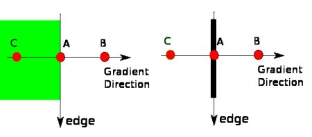
- Non-maximum Suppression After getting gradient magnitude and direction, a full scan of image is done to remove any unwanted pixels which may not constitute the edge. For this, at every pixel, pixel is checked if it is a local maximum in its neighborhood in the direction of gradient. Check the image below:


So what we finally get is strong edges in the image.
Canny Edge Detection in OpenCV
OpenCV puts all the above in single function, cv.Canny(). We will see how to use it. First argument is our input image. Second and third arguments are our minVal and maxVal respectively. Fourth argument is aperture_size. It is the size of Sobel kernel used for find image gradients. By default it is 3. Last argument is L2gradient which specifies the equation for finding gradient magnitude. If it is True, it uses the equation mentioned above which is more accurate, otherwise it uses this function: \(Edge\_Gradient \; (G) = |G_x| + |G_y|\). By default, it is False.
Python opencv cv2 canny
In this chapter, we will learn about
Theory
Canny Edge Detection is a popular edge detection algorithm. It was developed by John F. Canny in
- It is a multi-stage algorithm and we will go through each stages.
- Noise Reduction Since edge detection is susceptible to noise in the image, first step is to remove the noise in the image with a 5×5 Gaussian filter. We have already seen this in previous chapters.
- Finding Intensity Gradient of the Image Smoothened image is then filtered with a Sobel kernel in both horizontal and vertical direction to get first derivative in horizontal direction ( \(G_x\)) and vertical direction ( \(G_y\)). From these two images, we can find edge gradient and direction for each pixel as follows: \[ Edge\_Gradient \; (G) = \sqrt \\ Angle \; (\theta) = \tan^ \bigg(\frac\bigg) \] Gradient direction is always perpendicular to edges. It is rounded to one of four angles representing vertical, horizontal and two diagonal directions.
- Non-maximum Suppression After getting gradient magnitude and direction, a full scan of image is done to remove any unwanted pixels which may not constitute the edge. For this, at every pixel, pixel is checked if it is a local maximum in its neighborhood in the direction of gradient. Check the image below:
So what we finally get is strong edges in the image.
Canny Edge Detection in OpenCV
OpenCV puts all the above in single function, cv.Canny(). We will see how to use it. First argument is our input image. Second and third arguments are our minVal and maxVal respectively. Fourth argument is aperture_size. It is the size of Sobel kernel used for find image gradients. By default it is 3. Last argument is L2gradient which specifies the equation for finding gradient magnitude. If it is True, it uses the equation mentioned above which is more accurate, otherwise it uses this function: \(Edge\_Gradient \; (G) = |G_x| + |G_y|\). By default, it is False.
OpenCV Edge Detection in Python with cv2.Canny()

Edge detection is something we do naturally, but isn’t as easy when it comes to defining rules for computers. While various methods have been devised, the reigning method was developed by John F. Canny in 1986., and is aptly named the Canny method.
It’s fast, fairly robust, and works just about the best it could work for the type of technique it is. By the end of the guide, you’ll know how to perform real-time edge detection on videos, and produce something along the lines of:
Canny Edge Detection
What is the Canny method? It consists of four distinct operations:
- Gaussian smoothing
- Computing gradients
- Non-Max Suppression
- Hysteresis Thresholding
Gaussian smoothing is used as the first step to «iron out» the input image, and soften the noise, making the final output much cleaner.
Image gradients have been in use in earlier applications for edge detection. Most notably, Sobel and Scharr filters rely on image gradients. The Sobel filter boils down to two kernels (Gx and Gy), where Gx detects horizontal changes, while Gy detects vertical changes:
G x = [ − 1 0 + 1 − 2 0 + 2 − 1 0 + 1 ] G y = [ − 1 − 2 − 1 0 0 0 + 1 + 2 + 1 ]
When you slide them over an image, they’ll each «pick up» (emphasize) the lines in their respective orientation. Scharr kernels work in the same way, with different values:
G x = [ + 3 0 − 3 + 10 0 − 10 + 3 0 − 3 ] G y = [ + 3 + 10 + 3 0 0 0 − 3 − 10 − 3 ]
These filters, once convolved over the image, will produce feature maps:
Image credit: Davidwkennedy
For these feature maps, you can compute the gradient magnitude and gradient orientation — i.e. how intense the change is (how likely it is that something is an edge) and in which direction the change is pointing. Since Gy denotes the vertical change (Y-gradient), and Gx denotes the horizontal change (X-gradient) — you can calculate the magnitude by simply applying the Pythagorean theorem, to get the hypotenuse of the triangle formed by the «left» and «right» directions:
Using the magnitude and orientation, you can produce an image with its edged highlighted:
Image credit: Davidwkennedy
However — you can see how much noise was also caught from the texture of the bricks! Image gradients are very sensitive to noise. This is why Sobel and Scharr filters were used as the component, but not the only approach in Canny’s method. Gaussian smoothing helps here as well.
Non-Max Suppression
A noticeable issue with the Sobel filter is that edges aren’t really clear. It’s not like someone took a pencil and drew a line to create a line art of the image. The edges usually aren’t so clear cut in images, as light diffuses gradually. However, we can find the common line in the edges, and suppress the rest of the pixels around it, yielding a clean, thin separation line instead. This is known as Non-Max Suppression! The non-max pixels (ones smaller than the one we’re comparing them to in a small local field, such as a 3×3 kernel) get suppressed. The concept is applicable to more tasks than this, but let’s bind it to this context for now.
Hysteresis Thresholding
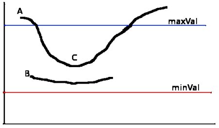
Many non-edges can and likely will be evaluated as edges, due to lighting conditions, the materials in the image, etc. Because of the various reasons these miscalculations occur — it’s hard to make an automated evaluation of what an edge certainly is and isn’t. You can threshold gradients, and only include the stronger ones, assuming that «real» edges are more intense than «fake» edges.
Thresholding works in much the same way as usual — if the gradient is below a lower threshold, remove it (zero it out), and if it’s above a given top threshold, keep it. Everything in-between the lower bound and upper bound is in the «gray zone». If any edge in-between the thresholds is connected to a definitive edge (ones above the threshold) — they’re also considered edges. If they’re not connected, they’re likely artifacts of a miscalculated edge.
That’s hysteresis thresholding! In effect, it helps clean up the final output and remove false edges, depending on what you classify as a false edge. To find good threshold values, you’ll generally experiment with different lower and upper bounds for the thresholds, or employ an automated method such as Otsu’s method or the Triangle method.
Let’s load an image in and grayscale it (Canny, just as Sobel/Scharr requires images to be gray-scaled):
import cv2 import matplotlib.pyplot as plt img = cv2.imread('finger.jpg', cv2.IMREAD_GRAYSCALE) img_blur = cv2.GaussianBlur(img, (3,3), 0) plt.imshow(img_blur, cmap='gray') The closeup image of a finger will serve as a good testing ground for edge detection — it’s not easy to discern a fingerprint from the image, but we can approximate one.
Edge Detection on Images with cv2.Canny()
Canny’s algorithm can be applied using OpenCV’s Canny() method:
cv2.Canny(input_img, lower_bound, upper_bound)