Python numpy произведение матриц

Базовые операции NumPy / np 3

Вы уже знаете, как создавать массив NumPy и как определять его элементы. Теперь пришло время разобраться с тем, как применять к ним различные операции.

Арифметические операторы

Арифметические операторы — первые, которые предстоит использовать. К числу наиболее очевидных относятся прибавление и умножение на скаляр.

>>> a = np.arange(4) >>> a array([0, 1, 2, 3]) >>> a+4 array([4, 5, 6, 7]) >>> a*2 array([0, 2, 4, 6]) 

Их можно использовать для двух массивов. В NumPy эти операции поэлементные, то есть, они применяются только к соответствующим друг другу элементам. Это должны быть объекты, которые занимают одно и то же положение, так что результатом станет новый массив, содержащий итоговые величины в тех же местах, что и операнды.

>>> b = np.arange(4,8) >>> b array([4, 5, 6, 7]) >>> a + b array([ 4, 6, 8, 10]) >>> a – b array([–4, –4, –4, –4]) >>> a * b array([ 0, 5, 12, 21]) 

Более того, эти операторы доступны и для функций, если те возвращают массив NumPy. Например, можно перемножить массив на синус или квадратный корень элементов массива b .

>>> a * np.sin(b) array([–0. , –0.95892427, –0.558831 , 1.9709598 ]) >>> a * np.sqrt(b) array([ 0. , 2.23606798, 4.89897949, 7.93725393]) 

И даже в случае с многомерными массивами можно применять арифметические операторы поэлементно.

>>> A = np.arange(0, 9).reshape(3, 3) >>> A array([[0, 1, 2], [3, 4, 5], [6, 7, 8]]) >>> B = np.ones((3, 3)) >>> B array([[ 1., 1., 1.], [ 1., 1., 1.], [ 1., 1., 1.]]) >>> A * B array([[ 0., 1., 2.], [ 3., 4., 5.], [ 6., 7., 8.]]) 

Произведение матриц

Выбор оператора для поэлементного применения — это странный аспект работы с библиотекой NumPy. В большинстве инструментов для анализа данных оператор * обозначает произведение матриц. Он применяется к обоим массивам. В NumPy же подобное произведение обозначается функцией dot() . Эта операция не поэлементная.

>>> np.dot(A,B) array([[ 3., 3., 3.], [ 12., 12., 12.], [ 21., 21., 21.]]) 

Каждый элемент результирующей матрицы — сумма произведений каждого элемента соответствующей строки в первой матрице с соответствующим элементом из колонки второй. Рисунок ниже показывает процесс произведения матриц (для двух элементов).

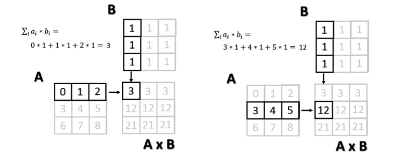
Еще один вариант записи произведения матриц — использование одной из двух матриц в качестве объекта функции dot() .

>>> A.dot(B) array([[ 3., 3., 3.], [ 12., 12., 12.], [ 21., 21., 21.]]) 

Но поскольку произведение матриц — это не коммутативная операция, порядок операндов имеет значение. В данном случае A*B не равняется B*A.

>>> np.dot(B,A) array([[ 9., 12., 15.], [ 9., 12., 15.], [ 9., 12., 15.]]) 

Операторы инкремента и декремента

На самом деле, в Python таких операторов нет, поскольку нет операторов ++ или — . Для увеличения или уменьшения значения используются += и -= . Они не отличаются от предыдущих, но вместо создания нового массива с результатами присваивают новое значение тому же массиву.

>>> a = np.arange(4) >>> a array([0, 1, 2, 3]) >>> a += 1 >>> a array([1, 2, 3, 4]) >>> a –= 1 >>> a array([0, 1, 2, 3]) 

Таким образом использование этих операторов дает возможность получать более масштабные результаты, чем в случае с обычными операторами инкремента, увеличивающими значения на один. Их можно использовать в самых разных ситуациях. Например, они подходят для изменения значений без создания нового массива.

array([0, 1, 2, 3]) >>> a += 4 >>> a array([4, 5, 6, 7]) >>> a *= 2 >>> a array([ 8, 10, 12, 14]) 

Универсальные функции (ufunc)

Универсальная функция, известная также как ufunc , — это функция, которая применяется в массиве к каждому элементу. Это значит, что она воздействует на каждый элемент массива ввода, генерируя соответствующий результат в массив вывода. Финальный массив соответствует по размеру массиву ввода.

Под это определение подпадает множество математических и тригонометрических операций; например, вычисление квадратного корня с помощью sqrt() , логарифма с log() или синуса с sin() .

>>> a = np.arange(1, 5) >>> a array([1, 2, 3, 4]) >>> np.sqrt(a) array([ 1. , 1.41421356, 1.73205081, 2. ]) >>> np.log(a) array([ 0. , 0.69314718, 1.09861229, 1.38629436]) >>> np.sin(a) array([ 0.84147098, 0.90929743, 0.14112001, –0.7568025 ]) 

Многие функции уже реализованы в библиотеке NumPy.

Функции агрегации

Функции агрегации выполняют операцию на наборе значений, например, на массиве, и выдают один результат. Таким образом, сумма всех элементов массива — это результат работы функции агрегации. Многие из таких функций реализованы в классе ndarray .

>>> a = np.array([3.3, 4.5, 1.2, 5.7, 0.3]) >>> a.sum() 15.0 >>> a.min() 0.29999999999999999 >>> a.max() 5.7000000000000002 >>> a.mean() 3.0 >>> a.std() 2.0079840636817816 

Источник

Linear algebra ( numpy.linalg )#

The NumPy linear algebra functions rely on BLAS and LAPACK to provide efficient low level implementations of standard linear algebra algorithms. Those libraries may be provided by NumPy itself using C versions of a subset of their reference implementations but, when possible, highly optimized libraries that take advantage of specialized processor functionality are preferred. Examples of such libraries are OpenBLAS, MKL (TM), and ATLAS. Because those libraries are multithreaded and processor dependent, environmental variables and external packages such as threadpoolctl may be needed to control the number of threads or specify the processor architecture.

The SciPy library also contains a linalg submodule, and there is overlap in the functionality provided by the SciPy and NumPy submodules. SciPy contains functions not found in numpy.linalg , such as functions related to LU decomposition and the Schur decomposition, multiple ways of calculating the pseudoinverse, and matrix transcendentals such as the matrix logarithm. Some functions that exist in both have augmented functionality in scipy.linalg . For example, scipy.linalg.eig can take a second matrix argument for solving generalized eigenvalue problems. Some functions in NumPy, however, have more flexible broadcasting options. For example, numpy.linalg.solve can handle “stacked” arrays, while scipy.linalg.solve accepts only a single square array as its first argument.

The term matrix as it is used on this page indicates a 2d numpy.array object, and not a numpy.matrix object. The latter is no longer recommended, even for linear algebra. See the matrix object documentation for more information.

The @ operator#

Introduced in NumPy 1.10.0, the @ operator is preferable to other methods when computing the matrix product between 2d arrays. The numpy.matmul function implements the @ operator.

Matrix and vector products#

Dot product of two arrays.

Compute the dot product of two or more arrays in a single function call, while automatically selecting the fastest evaluation order.

Return the dot product of two vectors.

Inner product of two arrays.

Compute the outer product of two vectors.

Matrix product of two arrays.

Compute tensor dot product along specified axes.

einsum (subscripts, *operands[, out, dtype, . ])

Evaluates the Einstein summation convention on the operands.

einsum_path (subscripts, *operands[, optimize])

Evaluates the lowest cost contraction order for an einsum expression by considering the creation of intermediate arrays.

Raise a square matrix to the (integer) power n.

Kronecker product of two arrays.

Decompositions#

Compute the qr factorization of a matrix.

linalg.svd (a[, full_matrices, compute_uv, . ])

Singular Value Decomposition.

Matrix eigenvalues#

Compute the eigenvalues and right eigenvectors of a square array.

Return the eigenvalues and eigenvectors of a complex Hermitian (conjugate symmetric) or a real symmetric matrix.

Compute the eigenvalues of a general matrix.

Compute the eigenvalues of a complex Hermitian or real symmetric matrix.

Norms and other numbers#

Compute the condition number of a matrix.

Compute the determinant of an array.

Return matrix rank of array using SVD method

Compute the sign and (natural) logarithm of the determinant of an array.

trace (a[, offset, axis1, axis2, dtype, out])

Return the sum along diagonals of the array.

Solving equations and inverting matrices#

Solve a linear matrix equation, or system of linear scalar equations.

Solve the tensor equation a x = b for x.

Return the least-squares solution to a linear matrix equation.

Compute the (multiplicative) inverse of a matrix.

Compute the (Moore-Penrose) pseudo-inverse of a matrix.

Compute the ‘inverse’ of an N-dimensional array.

Exceptions#

Generic Python-exception-derived object raised by linalg functions.

Linear algebra on several matrices at once#

Several of the linear algebra routines listed above are able to compute results for several matrices at once, if they are stacked into the same array.

This is indicated in the documentation via input parameter specifications such as a : (. M, M) array_like . This means that if for instance given an input array a.shape == (N, M, M) , it is interpreted as a “stack” of N matrices, each of size M-by-M. Similar specification applies to return values, for instance the determinant has det : (. ) and will in this case return an array of shape det(a).shape == (N,) . This generalizes to linear algebra operations on higher-dimensional arrays: the last 1 or 2 dimensions of a multidimensional array are interpreted as vectors or matrices, as appropriate for each operation.

Источник

numpy.matmul#

A location into which the result is stored. If provided, it must have a shape that matches the signature (n,k),(k,m)->(n,m). If not provided or None, a freshly-allocated array is returned.

For other keyword-only arguments, see the ufunc docs .

New in version 1.16: Now handles ufunc kwargs

The matrix product of the inputs. This is a scalar only when both x1, x2 are 1-d vectors.

If the last dimension of x1 is not the same size as the second-to-last dimension of x2.

If a scalar value is passed in.

Complex-conjugating dot product.

Sum products over arbitrary axes.

Einstein summation convention.

alternative matrix product with different broadcasting rules.

The behavior depends on the arguments in the following way.

• If both arguments are 2-D they are multiplied like conventional matrices.
• If either argument is N-D, N > 2, it is treated as a stack of matrices residing in the last two indexes and broadcast accordingly.
• If the first argument is 1-D, it is promoted to a matrix by prepending a 1 to its dimensions. After matrix multiplication the prepended 1 is removed.
• If the second argument is 1-D, it is promoted to a matrix by appending a 1 to its dimensions. After matrix multiplication the appended 1 is removed.

matmul differs from dot in two important ways:

• Multiplication by scalars is not allowed, use * instead.
• Stacks of matrices are broadcast together as if the matrices were elements, respecting the signature (n,k),(k,m)->(n,m) :

>>> a = np.ones([9, 5, 7, 4]) >>> c = np.ones([9, 5, 4, 3]) >>> np.dot(a, c).shape (9, 5, 7, 9, 5, 3) >>> np.matmul(a, c).shape (9, 5, 7, 3) >>> # n is 7, k is 4, m is 3 

The matmul function implements the semantics of the @ operator introduced in Python 3.5 following PEP 465.

It uses an optimized BLAS library when possible (see numpy.linalg ).

For 2-D arrays it is the matrix product:

>>> a = np.array([[1, 0], . [0, 1]]) >>> b = np.array([[4, 1], . [2, 2]]) >>> np.matmul(a, b) array([[4, 1], [2, 2]]) 

For 2-D mixed with 1-D, the result is the usual.

>>> a = np.array([[1, 0], . [0, 1]]) >>> b = np.array([1, 2]) >>> np.matmul(a, b) array([1, 2]) >>> np.matmul(b, a) array([1, 2]) 

Broadcasting is conventional for stacks of arrays

>>> a = np.arange(2 * 2 * 4).reshape((2, 2, 4)) >>> b = np.arange(2 * 2 * 4).reshape((2, 4, 2)) >>> np.matmul(a,b).shape (2, 2, 2) >>> np.matmul(a, b)[0, 1, 1] 98 >>> sum(a[0, 1, :] * b[0 , :, 1]) 98 

Vector, vector returns the scalar inner product, but neither argument is complex-conjugated:

Scalar multiplication raises an error.

>>> np.matmul([1,2], 3) Traceback (most recent call last): . ValueError: matmul: Input operand 1 does not have enough dimensions . 

The @ operator can be used as a shorthand for np.matmul on ndarrays.

>>> x1 = np.array([2j, 3j]) >>> x2 = np.array([2j, 3j]) >>> x1 @ x2 (-13+0j) 

Источник