Python neural network tensorflow

Сверточная нейронная сеть (CNN)

Оптимизируйте свои подборки Сохраняйте и классифицируйте контент в соответствии со своими настройками.

В этом руководстве показано обучение простой сверточной нейронной сети (CNN) для классификации изображений CIFAR . Поскольку в этом руководстве используется Keras Sequential API , для создания и обучения вашей модели потребуется всего несколько строк кода.

Импорт TensorFlow

import tensorflow as tf from tensorflow.keras import datasets, layers, models import matplotlib.pyplot as plt 

Загрузите и подготовьте набор данных CIFAR10.

Набор данных CIFAR10 содержит 60 000 цветных изображений в 10 классах, по 6 000 изображений в каждом классе. Набор данных разделен на 50 000 обучающих изображений и 10 000 тестовых изображений. Классы взаимоисключающие и между ними нет пересечения.

(train_images, train_labels), (test_images, test_labels) = datasets.cifar10.load_data() # Normalize pixel values to be between 0 and 1 train_images, test_images = train_images / 255.0, test_images / 255.0 

Downloading data from https://www.cs.toronto.edu/~kriz/cifar-10-python.tar.gz 170500096/170498071 [==============================] - 11s 0us/step 170508288/170498071 [==============================] - 11s 0us/step

Проверьте данные

Чтобы убедиться, что набор данных выглядит правильно, давайте построим первые 25 изображений из обучающего набора и отобразим имя класса под каждым изображением:

class_names = ['airplane', 'automobile', 'bird', 'cat', 'deer', 'dog', 'frog', 'horse', 'ship', 'truck'] plt.figure(figsize=(10,10)) for i in range(25): plt.subplot(5,5,i+1) plt.xticks([]) plt.yticks([]) plt.grid(False) plt.imshow(train_images[i]) # The CIFAR labels happen to be arrays, # which is why you need the extra index plt.xlabel(class_names[train_labels[i][0]]) plt.show()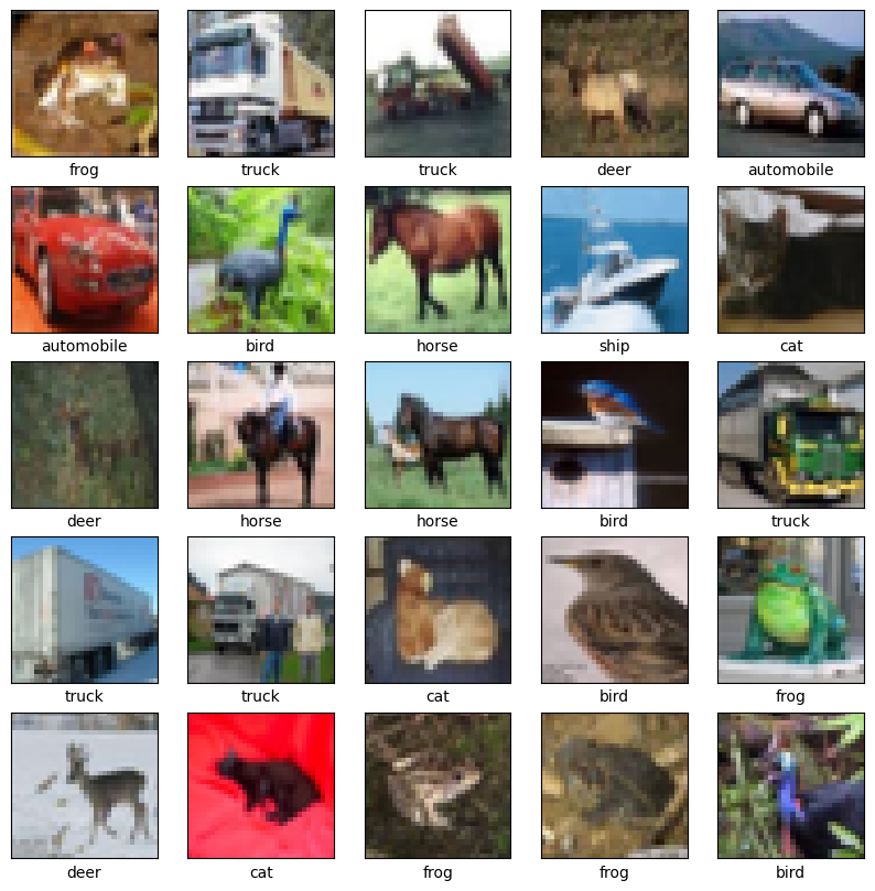 

Создание сверточной базы

6 строк кода ниже определяют основу свертки, используя общий шаблон: стек слоев Conv2D и MaxPooling2D .

В качестве входных данных CNN принимает тензоры формы (image_height, image_width, color_channels), игнорируя размер пакета. Если вы новичок в этих измерениях, color_channels относится к (R, G, B). В этом примере вы настроите свою CNN для обработки входных данных формы (32, 32, 3), которая является форматом изображений CIFAR. Вы можете сделать это, передав аргумент input_shape вашему первому слою.

model = models.Sequential() model.add(layers.Conv2D(32, (3, 3), activation='relu', input_shape=(32, 32, 3))) model.add(layers.MaxPooling2D((2, 2))) model.add(layers.Conv2D(64, (3, 3), activation='relu')) model.add(layers.MaxPooling2D((2, 2))) model.add(layers.Conv2D(64, (3, 3), activation='relu')) 

Давайте покажем архитектуру вашей модели на данный момент:

Model: "sequential" _________________________________________________________________ Layer (type) Output Shape Param # ================================================================= conv2d (Conv2D) (None, 30, 30, 32) 896 max_pooling2d (MaxPooling2D (None, 15, 15, 32) 0 ) conv2d_1 (Conv2D) (None, 13, 13, 64) 18496 max_pooling2d_1 (MaxPooling (None, 6, 6, 64) 0 2D) conv2d_2 (Conv2D) (None, 4, 4, 64) 36928 ================================================================= Total params: 56,320 Trainable params: 56,320 Non-trainable params: 0 _________________________________________________________________

Выше вы можете видеть, что выходные данные каждого слоя Conv2D и MaxPooling2D представляют собой трехмерный тензор формы (высота, ширина, каналы). Размеры ширины и высоты имеют тенденцию уменьшаться по мере того, как вы углубляетесь в сеть. Количество выходных каналов для каждого слоя Conv2D управляется первым аргументом (например, 32 или 64). Как правило, по мере уменьшения ширины и высоты вы можете позволить (вычислительно) добавить больше выходных каналов в каждый слой Conv2D.

Добавьте плотные слои сверху

Чтобы завершить модель, вы передадите последний выходной тензор из сверточной базы (формы (4, 4, 64)) в один или несколько плотных слоев для выполнения классификации. Плотные слои принимают в качестве входных данных векторы (которые являются одномерными), а текущий вывод представляет собой трехмерный тензор. Сначала вы сгладите (или развернете) 3D-выход в 1D, а затем добавите один или несколько плотных слоев сверху. CIFAR имеет 10 выходных классов, поэтому вы используете последний плотный слой с 10 выходными данными.

model.add(layers.Flatten()) model.add(layers.Dense(64, activation='relu')) model.add(layers.Dense(10)) 

Вот полная архитектура вашей модели:

Model: "sequential" _________________________________________________________________ Layer (type) Output Shape Param # ================================================================= conv2d (Conv2D) (None, 30, 30, 32) 896 max_pooling2d (MaxPooling2D (None, 15, 15, 32) 0 ) conv2d_1 (Conv2D) (None, 13, 13, 64) 18496 max_pooling2d_1 (MaxPooling (None, 6, 6, 64) 0 2D) conv2d_2 (Conv2D) (None, 4, 4, 64) 36928 flatten (Flatten) (None, 1024) 0 dense (Dense) (None, 64) 65600 dense_1 (Dense) (None, 10) 650 ================================================================= Total params: 122,570 Trainable params: 122,570 Non-trainable params: 0 _________________________________________________________________

Сводка по сети показывает, что выходные данные (4, 4, 64) были сглажены в векторы формы (1024) перед прохождением через два плотных слоя.

Скомпилируйте и обучите модель

model.compile(optimizer='adam', loss=tf.keras.losses.SparseCategoricalCrossentropy(from_logits=True), metrics=['accuracy']) history = model.fit(train_images, train_labels, epochs=10, validation_data=(test_images, test_labels)) 

Epoch 1/10 1563/1563 [==============================] - 8s 4ms/step - loss: 1.4971 - accuracy: 0.4553 - val_loss: 1.2659 - val_accuracy: 0.5492 Epoch 2/10 1563/1563 [==============================] - 6s 4ms/step - loss: 1.1424 - accuracy: 0.5966 - val_loss: 1.1025 - val_accuracy: 0.6098 Epoch 3/10 1563/1563 [==============================] - 6s 4ms/step - loss: 0.9885 - accuracy: 0.6539 - val_loss: 0.9557 - val_accuracy: 0.6629 Epoch 4/10 1563/1563 [==============================] - 6s 4ms/step - loss: 0.8932 - accuracy: 0.6878 - val_loss: 0.8924 - val_accuracy: 0.6935 Epoch 5/10 1563/1563 [==============================] - 6s 4ms/step - loss: 0.8222 - accuracy: 0.7130 - val_loss: 0.8679 - val_accuracy: 0.7025 Epoch 6/10 1563/1563 [==============================] - 6s 4ms/step - loss: 0.7663 - accuracy: 0.7323 - val_loss: 0.9336 - val_accuracy: 0.6819 Epoch 7/10 1563/1563 [==============================] - 6s 4ms/step - loss: 0.7224 - accuracy: 0.7466 - val_loss: 0.8546 - val_accuracy: 0.7086 Epoch 8/10 1563/1563 [==============================] - 6s 4ms/step - loss: 0.6726 - accuracy: 0.7611 - val_loss: 0.8777 - val_accuracy: 0.7068 Epoch 9/10 1563/1563 [==============================] - 6s 4ms/step - loss: 0.6372 - accuracy: 0.7760 - val_loss: 0.8410 - val_accuracy: 0.7179 Epoch 10/10 1563/1563 [==============================] - 6s 4ms/step - loss: 0.6024 - accuracy: 0.7875 - val_loss: 0.8475 - val_accuracy: 0.7192

Оценить модель

plt.plot(history.history['accuracy'], label='accuracy') plt.plot(history.history['val_accuracy'], label = 'val_accuracy') plt.xlabel('Epoch') plt.ylabel('Accuracy') plt.ylim([0.5, 1]) plt.legend(loc='lower right') test_loss, test_acc = model.evaluate(test_images, test_labels, verbose=2) 

313/313 - 1s - loss: 0.8475 - accuracy: 0.7192 - 634ms/epoch - 2ms/step

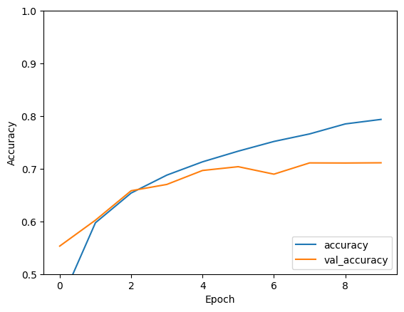
Ваша простая CNN достигла точности теста более 70%. Неплохо для нескольких строк кода! Для другого стиля CNN ознакомьтесь с примером быстрого запуска TensorFlow 2 для экспертов , в котором используется API подклассов Keras и tf.GradientTape .

Если не указано иное, контент на этой странице предоставляется по лицензии Creative Commons «С указанием авторства 4.0», а примеры кода – по лицензии Apache 2.0. Подробнее об этом написано в правилах сайта. Java – это зарегистрированный товарный знак корпорации Oracle и ее аффилированных лиц.

Последнее обновление: 2022-01-26 UTC.

Источник

Artificial Neural Network in TensorFlow

In this article, we are going to see some basics of ANN and a simple implementation of an artificial neural network. Tensorflow is a powerful machine learning library to create models and neural networks.

So, before we start What are Artificial neural networks? Here is a simple and clear definition of artificial neural networks. So long story in short artificial neural networks is a technology that mimics a human brain to learn from some key features and classify or predict in the real world. An artificial neural network is composed of numbers of neurons which is compared to the neurons in the human brain.

It is designed to make a computer learn from small insights and features and make them autonomous to learn from the real world and provide solutions in real-time faster than a human.

A neuron in an artificial neural network, will perform two operations inside it

So a basic Artificial neural network will be in a form of,

1. Input layer – To get the data from the user or a client or a server to analyze and give the result.
2. Hidden layers – This layer can be in any number and these layers will analyze the inputs with passing through them with different biases, weights, and activation functions to provide an output
3. Output Layer – This is where we can get the result from a neural network.

So as we know the outline of the neural networks, now we shall move to the important functions and methods that help a neural network to learn correctly from the data.

Note: Any neural network can learn from the data but without good parameter values a neural network might not able to learn from the data correctly and will not give you the correct result.

Some of the features that determine the quality of our neural network are:

Now we shall discuss each one of them in detail,

The first stage of our model building is:

Python3

Layers

Layers in a neural network are very important as we saw earlier an artificial neural network consists of 3 layers an input layer, hidden layer, output layer. The input layer consists of the features and values that need to be analyzed inside a neural network. Basically, this is a layer that will read our input features onto an Artificial neural network.

A hidden layer is a layer where all the magic happens when all the input neurons pass the features to the hidden layer with a weight and a bias each and every neuron inside the hidden layer will sum up all the weighted features from all the input layers and apply an activation function to keep the values between 0 and 1 for easier learning. Here we need to choose the number of neurons in each layer manually and it must be the best value for the network.

Here the real decision-makers are the weights between each layer which will finally pass a value of 0 to 1 to the output layer. Till this, we have seen the importance of each level of layers in an artificial neural network. There are many types of layers in TensorFlow but the one that we will use a lot is Dense

syntax: tf.keras.layers.Dense()

This is a fully connected layer in which each and every feature input will be connected somehow with the result.

Activation function

Activation functions are simply mathematical methods that bring all the values inside a range of 0 to 1 so that it will be very easier for the machine to learn the data in its process of analyzing the data. There are a variety of activation functions that are supported by the Tensor flow. Some of the commonly used functions are,

Each and every activation function has its own specific use cases and drawbacks. But the activation function that is used in the hidden and input layers is ‘Relu’ and another this which will have a greater impact on the result is losses.

After this, we can see the params in the compilation of the model in TensorFlow,

Источник