Python neural network backpropagation

A Step by Step Backpropagation Example

Backpropagation is a common method for training a neural network. There is no shortage of papers online that attempt to explain how backpropagation works, but few that include an example with actual numbers. This post is my attempt to explain how it works with a concrete example that folks can compare their own calculations to in order to ensure they understand backpropagation correctly.

Backpropagation in Python

You can play around with a Python script that I wrote that implements the backpropagation algorithm in this Github repo.

Backpropagation Visualization

For an interactive visualization showing a neural network as it learns, check out my Neural Network visualization.

Additional Resources

If you find this tutorial useful and want to continue learning about neural networks, machine learning, and deep learning, I highly recommend checking out Adrian Rosebrock’s new book, Deep Learning for Computer Vision with Python. I really enjoyed the book and will have a full review up soon.

Overview

For this tutorial, we’re going to use a neural network with two inputs, two hidden neurons, two output neurons. Additionally, the hidden and output neurons will include a bias.

Here’s the basic structure:

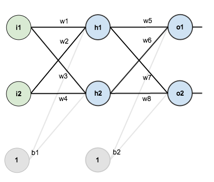
In order to have some numbers to work with, here are the initial weights , the biases , and training inputs/outputs :

The goal of backpropagation is to optimize the weights so that the neural network can learn how to correctly map arbitrary inputs to outputs.

For the rest of this tutorial we’re going to work with a single training set: given inputs 0.05 and 0.10, we want the neural network to output 0.01 and 0.99.

The Forward Pass

To begin, lets see what the neural network currently predicts given the weights and biases above and inputs of 0.05 and 0.10. To do this we’ll feed those inputs forward though the network.

We figure out the total net input to each hidden layer neuron, squash the total net input using an activation function (here we use the logistic function), then repeat the process with the output layer neurons.

Here’s how we calculate the total net input for :

We then squash it using the logistic function to get the output of :

Carrying out the same process for we get:

We repeat this process for the output layer neurons, using the output from the hidden layer neurons as inputs.

And carrying out the same process for we get:

Calculating the Total Error

We can now calculate the error for each output neuron using the squared error function and sum them to get the total error:

The is included so that exponent is cancelled when we differentiate later on. The result is eventually multiplied by a learning rate anyway so it doesn’t matter that we introduce a constant here [1].

For example, the target output for is 0.01 but the neural network output 0.75136507, therefore its error is:

Repeating this process for (remembering that the target is 0.99) we get:

The total error for the neural network is the sum of these errors:

The Backwards Pass

Our goal with backpropagation is to update each of the weights in the network so that they cause the actual output to be closer the target output, thereby minimizing the error for each output neuron and the network as a whole.

Output Layer

Consider . We want to know how much a change in affects the total error, aka .

is read as “the partial derivative of with respect to “. You can also say “the gradient with respect to “.

By applying the chain rule we know that:

Visually, here’s what we’re doing:

We need to figure out each piece in this equation.

First, how much does the total error change with respect to the output?

When we take the partial derivative of the total error with respect to , the quantity becomes zero because does not affect it which means we’re taking the derivative of a constant which is zero.

Next, how much does the output of change with respect to its total net input?

The partial derivative of the logistic function is the output multiplied by 1 minus the output:

Finally, how much does the total net input of change with respect to ?

You’ll often see this calculation combined in the form of the delta rule:

Alternatively, we have and which can be written as , aka (the Greek letter delta) aka the node delta. We can use this to rewrite the calculation above:

Some sources extract the negative sign from so it would be written as:

To decrease the error, we then subtract this value from the current weight (optionally multiplied by some learning rate, eta, which we’ll set to 0.5):

Some sources use (alpha) to represent the learning rate, others use (eta), and others even use (epsilon).

We can repeat this process to get the new weights , , and :

We perform the actual updates in the neural network after we have the new weights leading into the hidden layer neurons (ie, we use the original weights, not the updated weights, when we continue the backpropagation algorithm below).

Hidden Layer

Next, we’ll continue the backwards pass by calculating new values for , , , and .

Big picture, here’s what we need to figure out:

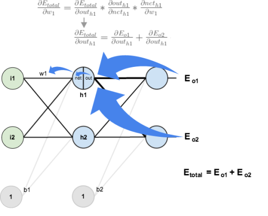
We’re going to use a similar process as we did for the output layer, but slightly different to account for the fact that the output of each hidden layer neuron contributes to the output (and therefore error) of multiple output neurons. We know that affects both and therefore the needs to take into consideration its effect on the both output neurons:

We can calculate using values we calculated earlier:

Following the same process for , we get:

Now that we have , we need to figure out and then for each weight:

We calculate the partial derivative of the total net input to with respect to the same as we did for the output neuron:

You might also see this written as:

Finally, we’ve updated all of our weights! When we fed forward the 0.05 and 0.1 inputs originally, the error on the network was 0.298371109. After this first round of backpropagation, the total error is now down to 0.291027924. It might not seem like much, but after repeating this process 10,000 times, for example, the error plummets to 0.0000351085. At this point, when we feed forward 0.05 and 0.1, the two outputs neurons generate 0.015912196 (vs 0.01 target) and 0.984065734 (vs 0.99 target).

If you’ve made it this far and found any errors in any of the above or can think of any ways to make it clearer for future readers, don’t hesitate to drop me a note. Thanks!

And while I have you…

In addition to dabbling in data science, I run Preceden timeline maker, the best timeline maker software on the web. If you ever need to create a high level timeline or roadmap to get organized or align your team, Preceden is a great option.

Share this:

Like this:

Related

1,056 thoughts on “ A Step by Step Backpropagation Example ”

Hi, it seems your network visualization is giving an error. numInputs not defined. Please, let me know when it is working, I’d like to check whether I can reference or include it into my materials.
Best
Ingo Dahn

Although this is a good post. I don’t think the writer understand about bias, that’s why there’s no concrete explanation about how to update bias in this post.

The author likely assigned the same bias for the hidden and output neurons for simplicity. The article does not show the step of updating the bias weights, presumably as it is the exact same process as is used to update other weights (it is actually simpler, since the bias node activation is always 1.)

Correct observation. The bias is not updated, therefore the total error in the first round and the second round goes like this:
Matt: E=0.298371109 -> E=0.291027924
If you correctly update the bias also, then it should be like this:
Barek: E=0.298371 -> E=0.280471
When I did not update the bias, just like Matt, then I got
Barek: E=0.298371 -> E=0.291028
This proves that Matt did not update the bias.
Anyway, this is a great post. Thank you, Matt!

Thanks to such the nice explanation!
I implement my first neural network by referring the post, thanks.

hello! If there are multiple hidden layers, say two, three, or even more; How do you continue the back-propagation? Do you always take it two layers at a time? If we are dealing with the leftmost hidden layer, do we need to track how changes to weights in this layer effect the following multiple hidden layers and then finally the output layer (working out error) Tracing all routes that changes in a far left weight effect error seems to “blow up” very quickly so to speak. Can anyone point me towards a worked example with at least 1 more hidden layer?

Hello Justin,
the back-propagation works also with multiple hidden layers.
You will find a good visualization for neural networks:
http://playground.tensorflow.org/
Sincerly
Albrecht

Thank you for your detailed explanation.
I wonder how you set the outputs to be 0.01 and 0.99 ?
It is arbitrary chosen? Does the amount of the inputs and their vaules impact of the decesion how to set the outputs?

This is multi-label classification, correct?
Otherwise I would be wondering why we don’t either use a softmax in the last layer? Also our outputs don’t sum to 1. Thank you and kind regards

Hmm, in my case, after first round of backpropagation the total error is 0.291027774 instead 0.291027924. And after repeating 10,000 times, the total error is 0.0000351019 instead 0.0000351085. Тhe rest of the calculations matched perfectly

Same, I wonder if that is my own issue or some floating point magic. The network seems to be learning…

I’m totally stumped, I’ve been over this article like 100 times and scrolled through as many comments and I cannot figure out how back propagation would work with multiple hidden layers. Using the example (I’m using d instead of the swirly thing because I’ve seen other comments do that and idk how to type the other character): dEtotal / dW1 = dEtotal / dOutputH1 * stuff I get
dEtotal / dOutputH1 = dEo1/dNeto1 + same for O2
dEo1/dNeto1 = dEo1 / dOutputo1 * dOutputo1 / dNeto1
dEo1 / dOutputo1 = -(targeto1 – outputo1) I understand that for the output layer, but if you have a second hidden layer in place of the output layer then for some hn dEhn / dOutputhn = -(targethn – outputhn)
What the hell is the target value? I’ve been pulling my hair out for like 4 hours and I cannot figure it out.

You need to work backwards through the layers and use the ‘delta’ from the next layer’s neurons. This delta should be stored whilst you are working backwards. The delta is the derivative of the current neurons output multiplied by the sum of all output neurons deltas * the weight between that neuron and the current one. So what you see in the blue box “You might also see this written as” works but replace input i, with the current neurons output passed through the derivative of the activation function

Источник

Deep Neural net with forward and back propagation from scratch – Python

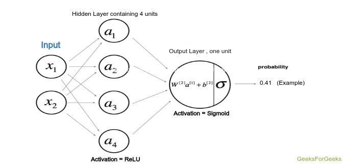
This article aims to implement a deep neural network from scratch. We will implement a deep neural network containing a hidden layer with four units and one output layer. The implementation will go from very scratch and the following steps will be implemented.
Algorithm:

1. Visualizing the input data 2. Deciding the shapes of Weight and bias matrix 3. Initializing matrix, function to be used 4. Implementing the forward propagation method 5. Implementing the cost calculation 6. Backpropagation and optimizing 7. prediction and visualizing the output

Architecture of the model:
The architecture of the model has been defined by the following figure where the hidden layer uses the Hyperbolic Tangent as the activation function while the output layer, being the classification problem uses the sigmoid function.

Weights and bias:
The weights and the bias that is going to be used for both the layers have to be declared initially and also among them the weights will be declared randomly in order to avoid the same output of all units, while the bias will be initialized to zero. The calculation will be done from the scratch itself and according to the rules given below where W1, W2 and b1, b2 are the weights and bias of first and second layer respectively. Here A stands for the activation of a particular layer.

Cost Function:
The cost function of the above model will pertain to the cost function used with logistic regression. Hence, in this tutorial we will be using the cost function:

Code: Visualizing the data

Источник