Python matplotlib pyplot bar

Matplotlib Bar chart

Matplotlib may be used to create bar charts. You might like the Matplotlib gallery.

Matplotlib is a python library for visualizing data. You can use it to create bar charts in python. Installation of matplot is on pypi, so just use pip: pip install matplotlib

The course below is all about data visualization:

Bar chart code

A bar chart shows values as vertical bars, where the position of each bar indicates the value it represents. matplot aims to make it as easy as possible to turn data into Bar Charts.

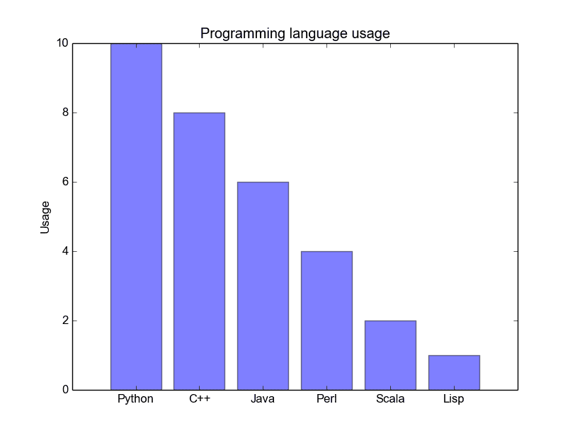
A bar chart in matplotlib made from python code. The code below creates a bar chart:

import matplotlib.pyplot as plt; plt.rcdefaults()
import numpy as np
import matplotlib.pyplot as plt

objects = (‘Python’, ‘C++’, ‘Java’, ‘Perl’, ‘Scala’, ‘Lisp’)
y_pos = np.arange(len(objects))
performance = [10,8,6,4,2,1]

plt.bar(y_pos, performance, align=‘center’, alpha=0.5)
plt.xticks(y_pos, objects)
plt.ylabel(‘Usage’)
plt.title(‘Programming language usage’)

plt.show()

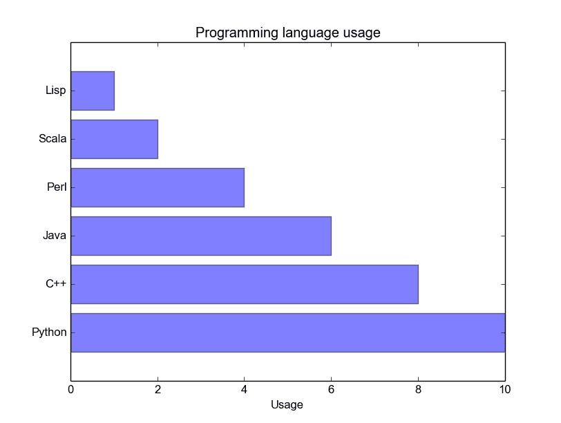
Matplotlib charts can be horizontal, to create a horizontal bar chart:

import matplotlib.pyplot as plt; plt.rcdefaults()
import numpy as np
import matplotlib.pyplot as plt

objects = (‘Python’, ‘C++’, ‘Java’, ‘Perl’, ‘Scala’, ‘Lisp’)
y_pos = np.arange(len(objects))
performance = [10,8,6,4,2,1]

plt.barh(y_pos, performance, align=‘center’, alpha=0.5)
plt.yticks(y_pos, objects)
plt.xlabel(‘Usage’)
plt.title(‘Programming language usage’)

plt.show()

Bar chart comparison

You can compare two data series using this Matplotlib code:

import numpy as np
import matplotlib.pyplot as plt

# data to plot
n_groups = 4
means_frank = (90, 55, 40, 65)
means_guido = (85, 62, 54, 20)

# create plot
fig, ax = plt.subplots()
index = np.arange(n_groups)
bar_width = 0.35
opacity = 0.8

rects1 = plt.bar(index, means_frank, bar_width,
alpha=opacity,
color=‘b’,
label=‘Frank’)

rects2 = plt.bar(index + bar_width, means_guido, bar_width,
alpha=opacity,
color=‘g’,
label=‘Guido’)

plt.xlabel(‘Person’)
plt.ylabel(‘Scores’)
plt.title(‘Scores by person’)
plt.xticks(index + bar_width, (‘A’, ‘B’, ‘C’, ‘D’))
plt.legend()

plt.tight_layout()
plt.show()

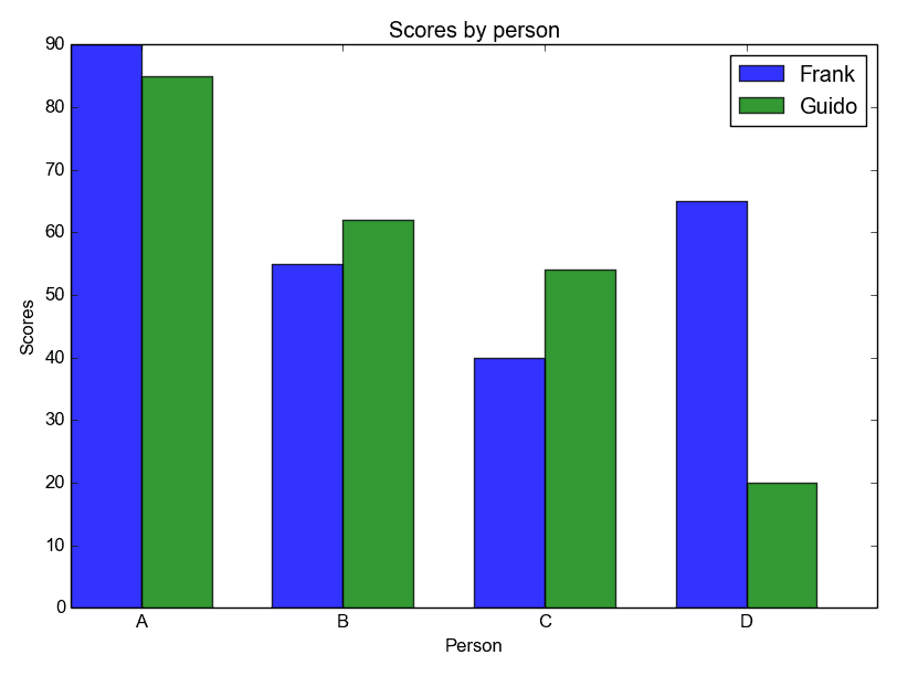
Python Bar Chart comparison

Stacked bar chart

The example below creates a stacked bar chart with Matplotlib. Stacked bar plots show diffrent groups together.

# load matplotlib
import matplotlib.pyplot as plt

# data set
x = [‘A’, ‘B’, ‘C’, ‘D’]
y1 = [100, 120, 110, 130]
y2 = [120, 125, 115, 125]

# plot stacked bar chart
plt.bar(x, y1, color=‘g’)
plt.bar(x, y2, bottom=y1, color=‘y’)
plt.show()

Источник

Matplotlib. Урок 4.3. Визуализация данных. Столбчатые и круговые диаграммы

В этому уроке изучим особенности работы со столбчатой и круговой диаграммами.

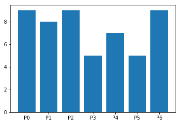
Столбчатые диаграммы

Для визуализации категориальных данных хорошо подходят столбчатые диаграммы. Для их построения используются функции:

bar() – для построения вертикальной диаграммы

barh() – для построения горизонтальной диаграммы.

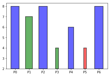
Построим простую диаграмму:

np.random.seed(123) groups = [f"P" for i in range(7)] counts = np.random.randint(3, 10, len(groups)) plt.bar(groups, counts)

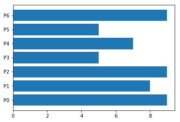
Если заменим bar() на barh() получим горизонтальную диаграмму:

Рассмотрим более подробно параметры функции bar() :

• x : набор величин
  • x координаты столбцов
  • Высоты столбцов
  • Ширина столбцов
  • y координата базы
  • Выравнивание по координате x .
  • color : скалярная величина, массив или optional
    • Цвет столбцов диаграммы
    • Цвет границы столбцов
    • Ширина границы
    • Метки для столбца
    • Величина ошибки для графика. Выставленное значение удаляется/прибавляется к верхней (правой – для горизонтального графика) границе. Может принимать следующие значения:
      • скаляр: симметрично +/- для всех баров
      • shape(N,) : симметрично +/- для каждого бара
      • shape(2,N) : выборочного – и + для каждого бара. Первая строка содержит нижние значения ошибок, вторая строка – верхние.
      • None : не отображать значения ошибок. Это значение используется по умолчанию.
      • Цвет линии ошибки.
      • Включение логарифмического масштаба для оси y
      • Ориентация: вертикальная или горизонтальная.

      Построим более сложный пример, демонстрирующий работу с параметрами:

      import matplotlib.colors as mcolors bc = mcolors.BASE_COLORS np.random.seed(123) groups = [f"P" for i in range(7)] counts = np.random.randint(0, len(bc), len(groups)) width = counts*0.1 colors = [["r", "b", "g"][int(np.random.randint(0, 3, 1))] for _ in counts] plt.bar(groups, counts, width=width, alpha=0.6, bottom=2, color=colors, edgecolor="k", linewidth=2)

      

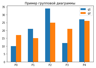
      Групповые столбчатые диаграммы

      Используя определенным образом подготовленные данные можно строить групповые диаграммы:

      cat_par = [f"P" for i in range(5)] g1 = [10, 21, 34, 12, 27] g2 = [17, 15, 25, 21, 26] width = 0.3 x = np.arange(len(cat_par)) fig, ax = plt.subplots() rects1 = ax.bar(x - width/2, g1, width, label='g1') rects2 = ax.bar(x + width/2, g2, width, label='g2') ax.set_title('Пример групповой диаграммы') ax.set_xticks(x) ax.set_xticklabels(cat_par) ax.legend()

      

      Диаграмма с errorbar элементом

      Errorbar элемент позволяет задать величину ошибки для каждого элемента графика. Для этого используются параметры xerr , yerr и ecolor (для задания цвета):

      np.random.seed(123) rnd = np.random.randint cat_par = [f"P" for i in range(5)] g1 = [10, 21, 34, 12, 27] error = np.array([[rnd(2,7),rnd(2,7)] for _ in range(len(cat_par))]).T fig, axs = plt.subplots(1, 2, figsize=(10, 5)) axs[0].bar(cat_par, g1, yerr=5, ecolor="r", alpha=0.5, edgecolor="b", linewidth=2) axs[1].bar(cat_par, g1, yerr=error, ecolor="r", alpha=0.5, edgecolor="b", linewidth=2)

      

      Круговые диаграммы

      Классическая круговая диаграмма

      Круговые диаграммы – это наглядный способ показать доли компонент в наборе. Они идеально подходят для отчетов, презентаций и т.п. Для построения круговых диаграмм в Matplotlib используется функция pie() .

      Пример построения диаграммы:

      vals = [24, 17, 53, 21, 35] labels = ["Ford", "Toyota", "BMV", "AUDI", "Jaguar"] fig, ax = plt.subplots() ax.pie(vals, labels=labels) ax.axis("equal")

      

      Рассмотрим параметры функции pie() :

      • x: массив
        • Массив с размерами долей.
        • Если параметр не равен None , то часть долей, который перечислены в передаваемом значении будут вынесены из диаграммы на заданное расстояние, пример диаграммы:

        

        • labels: list, optional , значение по умолчанию: None
          • Текстовые метки долей.
          • Цвета долей.
          • Формат текстовой метки внутри доли, текст – это численное значение показателя, связанного с конкретной долей.
          • Расстояние между центром каждой доли и началом текстовой метки, которая определяется параметром autopct .
          • Отображение тени для диаграммы.
          • Расстояние, на котором будут отображены текстовые метки долей. Если параметр равен None , то метки не будет отображены.
          • Задает угол, на который нужно повернуть диаграмму против часовой стрелке относительно оси x .
          • Величина радиуса диаграммы.
          • Определяет направление вращения – по часовой или против часовой стрелки.
          • Словарь параметров, определяющих внешний вид долей.
          • Словарь параметров определяющих внешний вид текстовых меток.
          • Центр диаграммы.
          • Если параметр равен True , то вокруг диаграммы будет отображена рамка.
          • Если параметр равен True , то текстовые метки будут повернуты на угол.

          Создадим пример, в котором продемонстрируем работу с параметрами функции pie() :

          vals = [24, 17, 53, 21, 35] labels = ["Ford", "Toyota", "BMV", "AUDI", "Jaguar"] explode = (0.1, 0, 0.15, 0, 0) fig, ax = plt.subplots() ax.pie(vals, labels=labels, autopct='%1.1f%%', shadow=True, explode=explode, wedgeprops=, rotatelabels=True) ax.axis("equal")

          

          Вложенные круговые диаграммы

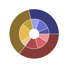
          Рассмотрим пример построения вложенной круговой диаграммы. Такая диаграмма состоит из двух компонент: внутренняя ее часть является детальным представлением информации, а внешняя – суммарную по заданным областям. Каждая область представляет собой список численных значений, вместе они образуют общий набор данных. Рассмотрим на примере:

          fig, ax = plt.subplots() offset=0.4 data = np.array([[5, 10, 7], [8, 15, 5], [11, 9, 7]]) cmap = plt.get_cmap("tab20b") b_colors = cmap(np.array([0, 8, 12])) sm_colors = cmap(np.array([1, 2, 3, 9, 10, 11, 13, 14, 15])) ax.pie(data.sum(axis=1), radius=1, colors=b_colors, wedgeprops=dict(width=offset, edgecolor='w')) ax.pie(data.flatten(), radius=1-offset, colors=sm_colors, wedgeprops=dict(width=offset, edgecolor='w'))

          

          Круговая диаграмма в виде бублика

          Построим круговую диаграмму в виде бублика (с отверстием посередине). Это можно сделать через параметр wedgeprops , который отвечает за внешний вид долей:

          vals = [24, 17, 53, 21, 35] labels = ["Ford", "Toyota", "BMV", "AUDI", "Jaguar"] fig, ax = plt.subplots() ax.pie(vals, labels=labels, wedgeprops=dict(width=0.5))

          

          P.S.

          Вводные уроки по “Линейной алгебре на Python” вы можете найти соответствующей странице нашего сайта . Все уроки по этой теме собраны в книге “Линейная алгебра на Python”.

          Если вам интересна тема анализа данных, то мы рекомендуем ознакомиться с библиотекой Pandas. Для начала вы можете познакомиться с вводными уроками. Все уроки по библиотеке Pandas собраны в книге “Pandas. Работа с данными”.

          Источник

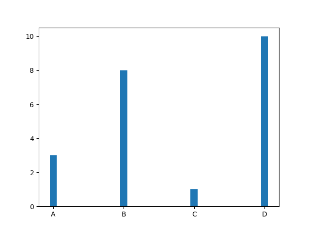
          Matplotlib Bars

          With Pyplot, you can use the bar() function to draw bar graphs:

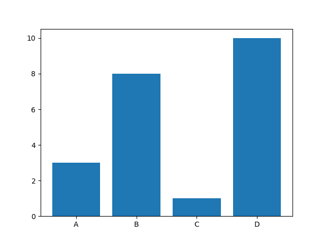
          Example

          import matplotlib.pyplot as plt
          import numpy as np

          x = np.array([«A», «B», «C», «D»])
          y = np.array([3, 8, 1, 10])

          Result:

          

          The bar() function takes arguments that describes the layout of the bars.

          The categories and their values represented by the first and second argument as arrays.

          Example

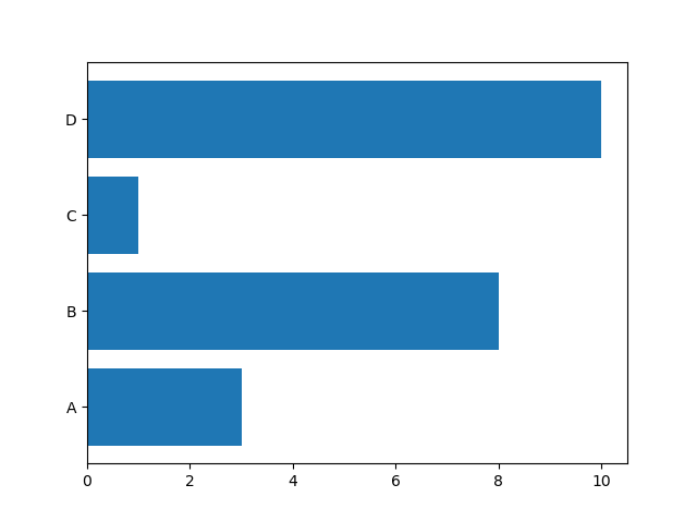
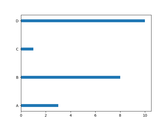
          Horizontal Bars

          If you want the bars to be displayed horizontally instead of vertically, use the barh() function:

          Example

          import matplotlib.pyplot as plt
          import numpy as np

          x = np.array([«A», «B», «C», «D»])
          y = np.array([3, 8, 1, 10])

          Result:

          

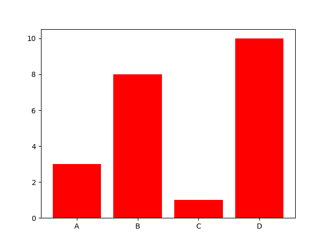
          Bar Color

          The bar() and barh() take the keyword argument color to set the color of the bars:

          Example

          import matplotlib.pyplot as plt
          import numpy as np

          x = np.array([«A», «B», «C», «D»])
          y = np.array([3, 8, 1, 10])

          plt.bar(x, y, color = «red»)
          plt.show()

          Result:

          

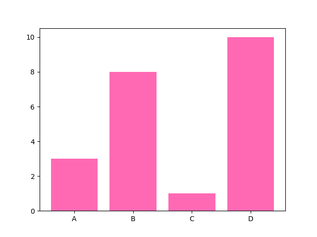
          Color Names

          Example

          import matplotlib.pyplot as plt
          import numpy as np

          x = np.array([«A», «B», «C», «D»])
          y = np.array([3, 8, 1, 10])

          plt.bar(x, y, color = «hotpink»)
          plt.show()

          Result:

          

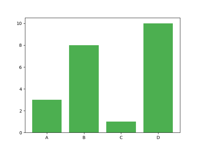
          Color Hex

          Example

          Draw 4 bars with a beautiful green color:

          import matplotlib.pyplot as plt
          import numpy as np

          x = np.array([«A», «B», «C», «D»])
          y = np.array([3, 8, 1, 10])

          plt.bar(x, y, color = «#4CAF50»)
          plt.show()

          Result:

          

          Bar Width

          The bar() takes the keyword argument width to set the width of the bars:

          Example

          import matplotlib.pyplot as plt
          import numpy as np

          x = np.array([«A», «B», «C», «D»])
          y = np.array([3, 8, 1, 10])

          plt.bar(x, y, width = 0.1)
          plt.show()

          Result:

          

          The default width value is 0.8

          Note: For horizontal bars, use height instead of width .

          Bar Height

          The barh() takes the keyword argument height to set the height of the bars:

          Example

          import matplotlib.pyplot as plt
          import numpy as np

          x = np.array([«A», «B», «C», «D»])
          y = np.array([3, 8, 1, 10])

          plt.barh(x, y, height = 0.1)
          plt.show()

          Result:

          

          The default height value is 0.8

          

          COLOR PICKER

          

          

          Report Error

          If you want to report an error, or if you want to make a suggestion, do not hesitate to send us an e-mail:

          Thank You For Helping Us!

          Your message has been sent to W3Schools.

          Top Tutorials

          Top References

          Top Examples

          Get Certified

          W3Schools is optimized for learning and training. Examples might be simplified to improve reading and learning. Tutorials, references, and examples are constantly reviewed to avoid errors, but we cannot warrant full correctness of all content. While using W3Schools, you agree to have read and accepted our terms of use, cookie and privacy policy.

          Источник

          Читайте также:  Java regexp space symbol