Python matplotlib plot from file

Plotting data from a file¶

Plotting data from a file is actually a two-step process.

pyplot.plotfile tried to do both at once. But each of the steps has so many possible variations and parameters that it does not make sense to squeeze both into a single function. Therefore, pyplot.plotfile has been deprecated.

The recommended way of plotting data from a file is therefore to use dedicated functions such as numpy.loadtxt or pandas.read_csv to read the data. These are more powerful and faster. Then plot the obtained data using matplotlib.

Note that pandas.DataFrame.plot is a convenient wrapper around Matplotlib to create simple plots.

import matplotlib.pyplot as plt import matplotlib.cbook as cbook import numpy as np import pandas as pd 

Using pandas¶

Subsequent are a few examples of how to replace plotfile with pandas . All examples need the the pandas.read_csv call first. Note that you can use the filename directly as a parameter:

The following slightly more involved pandas.read_csv call is only to make automatic rendering of the example work:

fname = cbook.get_sample_data('msft.csv', asfileobj=False) with cbook.get_sample_data('msft.csv') as file: msft = pd.read_csv(file) 

When working with dates, additionally call pandas.plotting.register_matplotlib_converters and use the parse_dates argument of pandas.read_csv :

pd.plotting.register_matplotlib_converters()

with cbook.get_sample_data(‘msft.csv’) as file: msft = pd.read_csv(file, parse_dates=[‘Date’])

Use indices¶

# Deprecated: plt.plotfile(fname, (0, 5, 6)) # Use instead: msft.plot(0, [5, 6], subplots=True) 

Use names¶

# Deprecated: plt.plotfile(fname, ('date', 'volume', 'adj_close')) # Use instead: msft.plot("Date", ["Volume", "Adj. Close*"], subplots=True) 

Use semilogy for volume¶

# Deprecated: plt.plotfile(fname, ('date', 'volume', 'adj_close'), plotfuncs='volume': 'semilogy'>) # Use instead: fig, axs = plt.subplots(2, sharex=True) msft.plot("Date", "Volume", ax=axs[0], logy=True) msft.plot("Date", "Adj. Close*", ax=axs[1]) 

Use semilogy for volume (by index)¶

# Deprecated: plt.plotfile(fname, (0, 5, 6), plotfuncs=5: 'semilogy'>) # Use instead: fig, axs = plt.subplots(2, sharex=True) msft.plot(0, 5, ax=axs[0], logy=True) msft.plot(0, 6, ax=axs[1]) 

Single subplot¶

# Deprecated: plt.plotfile(fname, ('date', 'open', 'high', 'low', 'close'), subplots=False) # Use instead: msft.plot("Date", ["Open", "High", "Low", "Close"]) 

Use bar for volume¶

# Deprecated: plt.plotfile(fname, (0, 5, 6), plotfuncs=5: "bar">) # Use instead: fig, axs = plt.subplots(2, sharex=True) axs[0].bar(msft.iloc[:, 0], msft.iloc[:, 5]) axs[1].plot(msft.iloc[:, 0], msft.iloc[:, 6]) fig.autofmt_xdate() 

Using numpy¶

fname2 = cbook.get_sample_data('data_x_x2_x3.csv', asfileobj=False) with cbook.get_sample_data('data_x_x2_x3.csv') as file: array = np.loadtxt(file) 

Labeling, if no names in csv-file¶

# Deprecated: plt.plotfile(fname2, cols=(0, 1, 2), delimiter=' ', names=['$x$', '$f(x)=x^2$', '$f(x)=x^3$']) # Use instead: fig, axs = plt.subplots(2, sharex=True) axs[0].plot(array[:, 0], array[:, 1]) axs[0].set(ylabel='$f(x)=x^2$') axs[1].plot(array[:, 0], array[:, 2]) axs[1].set(xlabel='$x$', ylabel='$f(x)=x^3$') 

More than one file per figure¶

# For simplicity of the example we reuse the same file. # In general they will be different. fname3 = fname2 # Depreacted: plt.plotfile(fname2, cols=(0, 1), delimiter=' ') plt.plotfile(fname3, cols=(0, 2), delimiter=' ', newfig=False) # use current figure plt.xlabel(r'$x$') plt.ylabel(r'$f(x) = x^2, x^3$') # Use instead: fig, ax = plt.subplots() ax.plot(array[:, 0], array[:, 1]) ax.plot(array[:, 0], array[:, 2]) ax.set(xlabel='$x$', ylabel='$f(x)=x^3$') plt.show() 

Keywords: matplotlib code example, codex, python plot, pyplot Gallery generated by Sphinx-Gallery

© Copyright 2002 — 2012 John Hunter, Darren Dale, Eric Firing, Michael Droettboom and the Matplotlib development team; 2012 — 2018 The Matplotlib development team.
Last updated on Jun 17, 2020. Created using Sphinx 3.1.1. Doc version v3.2.2-2-g137edd56a.

Источник

Plot data from excel file in matplotlib Python

This tutorial is the one in which you will learn a basic method required for data science. That skill is to plot the data from an excel file in matplotlib in Python. Here you will learn to plot data as a graph in the excel file using matplotlib and pandas in Python.

How to plot data from excel file using matplotlib?

Before we plot the data from excel file in matplotlib, first we have to take care of a few things.

• You must have these packages installed in your IDE:- matplotlib, pandas, xlrd.
• Save an Excel file on your computer in any easily accessible location.
• If you are doing this coding in command prompt or shell, then make sure your directories and packages are correctly managed.
• For the sake of simplicity, we will be doing this using any IDE available.

Step 1: Import the pandas and matplotlib libraries.

import pandas as pd import matplotlib.pyplot as plt

Step 2 : read the excel file using pd.read_excel( ‘ file location ‘) .

var = pd.read_excel('C:\\user\\name\\documents\\officefiles.xlsx') var.head()

To let the interpreter know that the following \ is to be ignored as the escape sequence, we use two \.
the “var” is the data frame name. To display the first five rows in pandas we use the data frame .head() function.

If you have multiple sheets, then to focus on one sheet we will mention that after reading the file location.

var = pd.read_excel('C:\\user\\name\\documents\\officefiles.xlsx','Sheet1') var.head()

Step 3: To select a given column or row.
Here you can select a specific range of rows and columns that you want to be displayed. Just by making a new list and mentioning the columns name.

varNew = var[['column1','column2','column3']] varNew.head()

To select data to be displayed after specific rows, use ‘skip rows’ attribute.

var = pd.read_excel('C:\\user\\name\\documents\\officefiles.xlsx', skiprows=6)

step 4: To plot the graph of the selected files column.
to plot the data just add plt.plot(varNew[‘column name’]) . Use plt.show() to plot the graph.

import matplotlib.pyplot as plt import pandas as pd var= pd.read_excel('C:\\Users\\name\\Documents\\officefiles.xlsx') plt.plot(var['column name']) var.head() plt.show()

You will get the Graph of the data as the output.

You may also love to learn:

Источник

Save a Plot to a File in Matplotlib (using 14 formats)

The Matplotlib is a popular plotting library for Python. It can be used in Python scripts and Jupyter Notebooks. The plot can be displayed in a separate window or a notebook. What if you would like to save the plot to a file? In this article, I will show you how to save the Matplotlib plot into a file. It can be done by using 14 different formats.

Quick code snippet

Below is a quick Python code snippet that shows how to save a figure to a file.

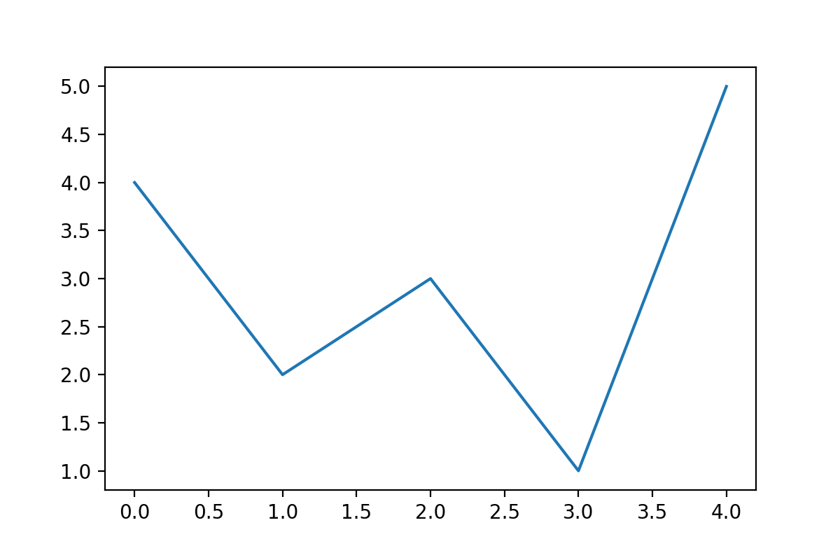
import matplotlib.pyplot as plt # create a plot plt.plot([4,2,3,1,5]) # save figure plt.savefig("my_plot.png") 

1. Please call plt.show() after plt.savefig() . Otherwise, you will get an empty plot in the file.
2. For Jupyter Notebook users, you need to call plt.savefig() in the same cell in which the plot is created. Otherwise, the file has an empty figure.

The savefig function — deep dive

All plots created with Matplotlib are saved with savefig function. Please take a while a look into savefig documentation.

Below are savefig arguments that you might find useful:

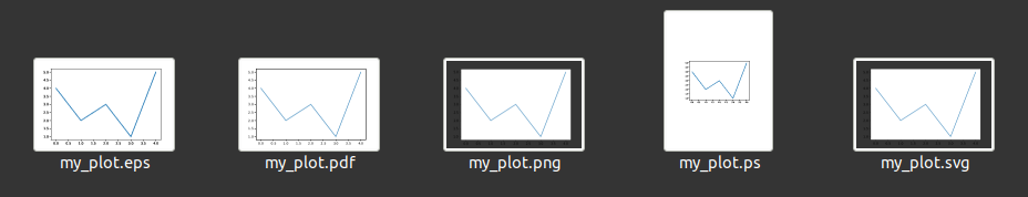
• fname — a path where to save a plot. It can be without extension. For fname with the extension included the format will be automatically selected. Common extensions: .png , .pdf , .svg ;
• dpi — a numeric value for dots per inch; it controls the size of the figure in pixels. You can read more in an article on how to change figure size in Matplotlib ;
• bbox_inches — controls the white space around the figure, if you don’t need margins, please set this parameter to tight ;
• transparent — is a boolean value that can turn the plot background into transparent;
• format — is a string with the output file format. Common formats are png , pdf , svg . If not specified, it is automatically set from the fname extension. The default is png .

You can list all available formats in Matplotlib with below Python code:

import matplotlib.pyplot as plt print(plt.gcf().canvas.get_supported_filetypes()) 

There are, in total 13 formats supported by Matplotlib .

Example of advanced save

Let’s try to save a figure to PNG format with transparent background with a size of 1200×800 pixels:

import matplotlib.pyplot as plt plt.figure(figsize=(6,4), dpi=200) plt.plot([4,2,3,1,5]) plt.savefig("my_plot.png", transparent=True) 

We set the size of the figure during creation, the size in pixels is computed by multiplying figsize by dpi .

Save Matplotlib figure

Earlier, we save plots in graphics formats. What if we would like to save the whole Matplotlib figure for further manipulation? It is possible. We can use the pickle library. It is a Python object serialization package. It doesn’t need to be installed additionally.

Here is an example Python code that creates the Matplitlib figure, saves to a file, and loads it back:

import pickle import matplotlib.pyplot as plt # create figure fig = plt.figure() plt.plot([4,2,3,1,5]) # save whole figure pickle.dump(fig, open("figure.pickle", "wb")) # load figure from file fig = pickle.load(open("figure.pickle", "rb")) 

Summary

You can save the Matplotlib plot to a file using 13 graphics formats. The most common formats are .png , .pdf , .svg and .jpg . The savefig() function has useful arguments: transparent , bbox_inches , or format . There is an option to serialize the figure object to a file and load it back with the pickle package. It can be used to save the figure for future manipulations.

Источник