Python комплексные числа сложение

cmath — Mathematical functions for complex numbers¶

This module provides access to mathematical functions for complex numbers. The functions in this module accept integers, floating-point numbers or complex numbers as arguments. They will also accept any Python object that has either a __complex__() or a __float__() method: these methods are used to convert the object to a complex or floating-point number, respectively, and the function is then applied to the result of the conversion.

For functions involving branch cuts, we have the problem of deciding how to define those functions on the cut itself. Following Kahan’s “Branch cuts for complex elementary functions” paper, as well as Annex G of C99 and later C standards, we use the sign of zero to distinguish one side of the branch cut from the other: for a branch cut along (a portion of) the real axis we look at the sign of the imaginary part, while for a branch cut along the imaginary axis we look at the sign of the real part.

For example, the cmath.sqrt() function has a branch cut along the negative real axis. An argument of complex(-2.0, -0.0) is treated as though it lies below the branch cut, and so gives a result on the negative imaginary axis:

>>> cmath.sqrt(complex(-2.0, -0.0)) -1.4142135623730951j 

But an argument of complex(-2.0, 0.0) is treated as though it lies above the branch cut:

>>> cmath.sqrt(complex(-2.0, 0.0)) 1.4142135623730951j 

Conversions to and from polar coordinates¶

A Python complex number z is stored internally using rectangular or Cartesian coordinates. It is completely determined by its real part z.real and its imaginary part z.imag . In other words:

Polar coordinates give an alternative way to represent a complex number. In polar coordinates, a complex number z is defined by the modulus r and the phase angle phi. The modulus r is the distance from z to the origin, while the phase phi is the counterclockwise angle, measured in radians, from the positive x-axis to the line segment that joins the origin to z.

The following functions can be used to convert from the native rectangular coordinates to polar coordinates and back.

Return the phase of x (also known as the argument of x), as a float. phase(x) is equivalent to math.atan2(x.imag, x.real) . The result lies in the range [-π, π], and the branch cut for this operation lies along the negative real axis. The sign of the result is the same as the sign of x.imag , even when x.imag is zero:

>>> phase(complex(-1.0, 0.0)) 3.141592653589793 >>> phase(complex(-1.0, -0.0)) -3.141592653589793 

The modulus (absolute value) of a complex number x can be computed using the built-in abs() function. There is no separate cmath module function for this operation.

Return the representation of x in polar coordinates. Returns a pair (r, phi) where r is the modulus of x and phi is the phase of x. polar(x) is equivalent to (abs(x), phase(x)) .

Return the complex number x with polar coordinates r and phi. Equivalent to r * (math.cos(phi) + math.sin(phi)*1j) .

Power and logarithmic functions¶

Return e raised to the power x, where e is the base of natural logarithms.

Returns the logarithm of x to the given base. If the base is not specified, returns the natural logarithm of x. There is one branch cut, from 0 along the negative real axis to -∞.

Return the base-10 logarithm of x. This has the same branch cut as log() .

Return the square root of x. This has the same branch cut as log() .

Trigonometric functions¶

Return the arc cosine of x. There are two branch cuts: One extends right from 1 along the real axis to ∞. The other extends left from -1 along the real axis to -∞.

Return the arc sine of x. This has the same branch cuts as acos() .

Return the arc tangent of x. There are two branch cuts: One extends from 1j along the imaginary axis to ∞j . The other extends from -1j along the imaginary axis to -∞j .

Hyperbolic functions¶

Return the inverse hyperbolic cosine of x. There is one branch cut, extending left from 1 along the real axis to -∞.

Return the inverse hyperbolic sine of x. There are two branch cuts: One extends from 1j along the imaginary axis to ∞j . The other extends from -1j along the imaginary axis to -∞j .

Return the inverse hyperbolic tangent of x. There are two branch cuts: One extends from 1 along the real axis to ∞ . The other extends from -1 along the real axis to -∞ .

Return the hyperbolic cosine of x.

Return the hyperbolic sine of x.

Return the hyperbolic tangent of x.

Classification functions¶

Return True if both the real and imaginary parts of x are finite, and False otherwise.

Return True if either the real or the imaginary part of x is an infinity, and False otherwise.

Return True if either the real or the imaginary part of x is a NaN, and False otherwise.

Return True if the values a and b are close to each other and False otherwise.

Whether or not two values are considered close is determined according to given absolute and relative tolerances.

rel_tol is the relative tolerance – it is the maximum allowed difference between a and b, relative to the larger absolute value of a or b. For example, to set a tolerance of 5%, pass rel_tol=0.05 . The default tolerance is 1e-09 , which assures that the two values are the same within about 9 decimal digits. rel_tol must be greater than zero.

abs_tol is the minimum absolute tolerance – useful for comparisons near zero. abs_tol must be at least zero.

The IEEE 754 special values of NaN , inf , and -inf will be handled according to IEEE rules. Specifically, NaN is not considered close to any other value, including NaN . inf and -inf are only considered close to themselves.

PEP 485 – A function for testing approximate equality

Constants¶

The mathematical constant π, as a float.

The mathematical constant e, as a float.

The mathematical constant τ, as a float.

Floating-point positive infinity. Equivalent to float(‘inf’) .

Complex number with zero real part and positive infinity imaginary part. Equivalent to complex(0.0, float(‘inf’)) .

A floating-point “not a number” (NaN) value. Equivalent to float(‘nan’) .

Complex number with zero real part and NaN imaginary part. Equivalent to complex(0.0, float(‘nan’)) .

Note that the selection of functions is similar, but not identical, to that in module math . The reason for having two modules is that some users aren’t interested in complex numbers, and perhaps don’t even know what they are. They would rather have math.sqrt(-1) raise an exception than return a complex number. Also note that the functions defined in cmath always return a complex number, even if the answer can be expressed as a real number (in which case the complex number has an imaginary part of zero).

A note on branch cuts: They are curves along which the given function fails to be continuous. They are a necessary feature of many complex functions. It is assumed that if you need to compute with complex functions, you will understand about branch cuts. Consult almost any (not too elementary) book on complex variables for enlightenment. For information of the proper choice of branch cuts for numerical purposes, a good reference should be the following:

Kahan, W: Branch cuts for complex elementary functions; or, Much ado about nothing’s sign bit. In Iserles, A., and Powell, M. (eds.), The state of the art in numerical analysis. Clarendon Press (1987) pp165–211.

Источник

Работа с числами в Python

В этом материале рассмотрим работу с числами в Python. Установите последнюю версию этого языка программирования и используйте IDE для работы с кодом, например, Visual Studio Code.

В Python достаточно просто работать с числами, ведь сам язык является простым и одновременно мощным. Он поддерживает всего три числовых типа:

Хотя int и float присутствуют в большинстве других языков программирования, наличие типа комплексных чисел — уникальная особенность Python. Теперь рассмотрим в деталях каждый из типов.

Целые и числа с плавающей точкой в Python

В программирование целые числа — это те, что лишены плавающей точкой, например, 1, 10, -1, 0 и так далее. Числа с плавающей точкой — это, например, 1.0, 6.1 и так далее.

Создание int и float чисел

Для создания целого числа нужно присвоить соответствующее значение переменной. Возьмем в качестве примера следующий код:

Здесь мы присваиваем значение 25 переменной var1 . Важно не использовать одинарные или двойные кавычки при создании чисел, поскольку они отвечают за представление строк. Рассмотрим следующий код.

В этих случаях данные представлены как строки, поэтому не могут быть обработаны так, как требуется. Для создания числа с плавающей точкой, типа float , нужно аналогичным образом присвоить значение переменной.

Здесь также не стоит использовать кавычки.

Проверить тип данных переменной можно с помощью встроенной функции type() . Можете проверить результат выполнения, скопировав этот код в свою IDE.

 
var1 = 1 # создание int 
var2 = 1.10 # создание float 
var3 = "1.10" # создание строки 
print(type(var1)) 
print(type(var2)) 
print(type(var3)) 
 
В Python также можно создавать крупные числа, но в таком случае нельзя использовать запятые.
 
 
# создание 1,000,000 
var1 = 1,000,000 # неправильно 
 
Если попытаться запустить этот код, то интерпретатор Python вернет ошибку. Для разделения значений целого числа используется нижнее подчеркивание. Вот пример корректного объявления.
 
 
# создание 1,000,000 
var1 = 1_000_000 # правильно 
print(var1) 
 
Значение выведем с помощью функции print :
 
Арифметические операции над целыми и числами с плавающей точкой
 
Используем такие арифметические операции, как сложение и вычитание, на числах. Для запуска этого кода откройте оболочку Python, введите python или python3 . Терминал должен выглядеть следующим образом:
 
 
Сложение
 
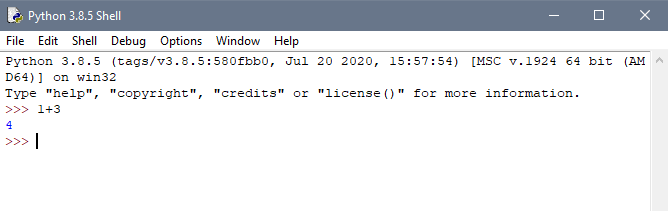
В Python сложение выполняется с помощью оператора + . В терминале Python выполните следующее.
 
Результатом будет сумма двух чисел, которая выведется в терминале.
 
 
Теперь запустим такой код.
 
В нем было выполнено сложение целого и числа с плавающей точкой. Можно обратить внимание на то, что результатом также является число с плавающей точкой. Таким образом сложение двух целых чисел дает целое число, но если хотя бы один из операндов является числом с плавающей точкой, то и результат станет такого же типа.
 
Вычитание
 
В Python для операции вычитания используется оператор -. Рассмотрим примеры.
 
>>> 3 - 1 2 >>> 1 - 5 -4 >>> 3.0 - 4.0 -1.0 >>> 3 - 1.0 2.0
 
Положительные числа получаются в случае вычитания маленького числа из более крупного. Если же из маленького наоборот вычесть большое, то результатом будет отрицательно число. По аналогии с операцией сложения при вычитании если один из операндов является числом с плавающей точкой, то и весь результат будет такого типа.
 
Умножение
 
Для умножения в Python применяется оператор * .
 
>>> 8 * 2 16 >>> 8.0 * 2 16.0 >>> 8.0 * 2.0 16.0
 
Если перемножить два целых числа, то результатом будет целое число. Если же использовать число с плавающей точкой, то результатом будет также число с плавающей точкой.
 
Деление
 
В Python деление выполняется с помощью оператора / .
 
>>> 3 / 1 3.0 >>> 4 / 2 2.0 >>> 3 / 2 1.5
 
В отличие от трех предыдущих операций при делении результатом всегда будет число с плавающей точкой. Также нужно помнить о том, что на 0 делить нельзя, иначе Python вернет ошибку ZeroDivisionError . Вот пример такого поведения.
 
>>> 1 / 0 Traceback (most recent call last): File "", line 1, in ZeroDivisionError: division by zero
 
Деление без остатка
 
При обычном делении с использованием оператора / результатом будет точное число с плавающей точкой. Но иногда достаточно получить лишь целую часть операции. Для этого есть операции интегрального деления. Стоит рассмотреть ее на примере.
 
Результатом такой операции становится частное. Остаток же можно получить с помощью модуля, о котором речь пойдет дальше.
 
Остаток от деления
 
Для получения остатка деления двух чисел используется оператор деления по модулю % .
 
>>> 5 % 2 1 >>> 4 % 2 0 >>> 3 % 2 1 >>> 5 % 3 2
 
На этих примерах видно, как это работает.
 
Возведение в степень
 
Число можно возвести в степень с помощью оператора ** .
 
Комплексные числа
 
Комплексные числа — это числа, которые включают мнимую часть. Python поддерживает их «из коробки». Их можно запросто создавать и использовать. Пример:
 
Источник