Python decompose time series

Advanced Time Series Analysis in Python: Seasonality and Trend Analysis (Decomposition), Autocorrelation

And other techniques to find relationships between multiple time series

Introduction

Following my very well-received post and Kaggle notebook on every single Pandas function to manipulate time series, it is time to take the trajectory of this TS project to visualization.

This post is about the core processes that make up an in-depth time series analysis. Specifically, we will talk about:

• Decomposition of time series — seasonality and trend analysis
• Analyzing and comparing multiple time series simultaneously
• Calculating autocorrelation and partial autocorrelation and what they represent

and if seasonality or trends among multiple series affect each other.

Most importantly, we will build some very cool visualizations, and this image should be a preview of what you will be learning.

I hope you are as excited about learning these things as I when writing this article. Let’s begin.

Read the notebook of the article here.

1. Decomposition of Time Series

Any time series distribution has 3 core components:

1. Seasonality — does the data have a clear cyclical/periodic pattern?
2. Trend — does the data represent a general upward or downward slope?
3. Noise — what are the outliers or missing values that are not consistent with the rest of the data?

Deconstructing a time series into these components is called decomposition, and we will explore each one in detail.

1.1 Seasonality analysis

Consider this TPS July Kaggle playground dataset:

Источник

Time Series Decomposition in Python

When working with time series data, we often want to decompose a time series into several components. We usually want to break out the trend, seasonility, and noise. In this article, we will learn how to decompose a time series in Python.

Data

Let’s load a data set of monthly milk production. We will load it from the url below. The data consists of monthly intervals and kilograms of milk produced.

import pandas as pd df = pd.read_csv('https://raw.githubusercontent.com/ourcodingclub/CC-time-series/master/monthly_milk.csv') df.month = pd.to_datetime(df.month) df = df.set_index('month') df.head()

milk_prod_per_cow_kg
month
1962-01-01	265.05
1962-02-01	252.45
1962-03-01	288.00
1962-04-01	295.20
1962-05-01	327.15

Decomposing

Let’s first plot our time series to see the trend.

To decompose a time series, we can use the seasonal_decompose from the statsmodels package. To decompose, we pass the variable we want to docompose and the type of model. You have to basic options, additive and multiplicable, here we use multiplicable.

from statsmodels.tsa.seasonal import seasonal_decompose result = seasonal_decompose(df.milk_prod_per_cow_kg, model = 'multiplicable')

Now the we have the result, we can plot the indiviual pieces of information. For example, below we plot the seasonal and trend.

We can also plot everything at once. For example, we can call plot on the result and it will plot each of the decoposed information.

Источник

6. Decomposing time series¶

Decomposing time series consists in extracting several time series from a time series. These extracted time series can represent different components, such as the trend, the seasonality or noise. These kinds of algorithms can be found in the pyts.decomposition module.

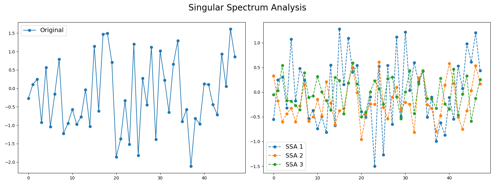
6.1. Singular Spectrum Analysis¶

SingularSpectrumAnalysis is an algorithm that decomposes a time series of length into several time series of length such that . The smaller the index , the more information about it contains. The higher the index , the more noise it contains. Taking the first extracted time series can be used as a preprocessing step to remove noise.

>>> from pyts.datasets import load_gunpoint >>> from pyts.decomposition import SingularSpectrumAnalysis >>> X, _, _, _ = load_gunpoint(return_X_y=True) >>> transformer = SingularSpectrumAnalysis(window_size=5) >>> X_new = transformer.transform(X) >>> X_new.shape (50, 5, 150) 

• N. Golyandina, and A. Zhigljavsky, “Singular Spectrum Analysis for Time Series”. Springer-Verlag Berlin Heidelberg (2013).

Источник