Python data analysis algorithms

Exploratory Data Analysis in Python

EDA is a phenomenon under data analysis used for gaining a better understanding of data aspects like:
– main features of data
– variables and relationships that hold between them
– identifying which variables are important for our problem
We shall look at various exploratory data analysis methods like:

• Descriptive Statistics, which is a way of giving a brief overview of the dataset we are dealing with, including some measures and features of the sample
• Grouping data [Basic grouping with group by]
• ANOVA, Analysis Of Variance, which is a computational method to divide variations in an observations set into different components.
• Correlation and correlation methods

The dataset we’ll be using is child voting dataset, which you can import in python as:

Python3

Descriptive Statistics

Descriptive statistics is a helpful way to understand characteristics of your data and to get a quick summary of it. Pandas in python provide an interesting method describe(). The describe function applies basic statistical computations on the dataset like extreme values, count of data points standard deviation etc. Any missing value or NaN value is automatically skipped. describe() function gives a good picture of distribution of data.

Python3

Here’s the output you’ll get on running above code:

Another useful method if value_counts() which can get count of each category in a categorical attributed series of values. For an instance suppose you are dealing with a dataset of customers who are divided as youth, medium and old categories under column name age and your dataframe is “DF”. You can run this statement to know how many people fall in respective categories. In our data set example education column can be used

Python3

The output of the above code will be:

One more useful tool is boxplot which you can use through matplotlib module. Boxplot is a pictorial representation of distribution of data which shows extreme values, median and quartiles. We can easily figure out outliers by using boxplots. Now consider the dataset we’ve been dealing with again and lets draw a boxplot on attribute population

Python3

DF = pd.read_csv( «https://raw.githubusercontent.com / fivethirtyeight / data / master / airline-safety / airline-safety.csv» )

The output plot would look like this with spotting out outliers:

Grouping data

Group by is an interesting measure available in pandas which can help us figure out effect of different categorical attributes on other data variables. Let’s see an example on the same dataset where we want to figure out affect of people’s age and education on the voting dataset.

Python3

The output would be somewhat like this:

If this group by output table is less understandable further analysts use pivot tables and heat maps for visualization on them.

ANOVA

ANOVA stands for Analysis of Variance. It is performed to figure out the relation between the different group of categorical data.
Under ANOVA we have two measures as result:
– F-testscore : which shows the variation of groups mean over variation
– p-value: it shows the importance of the result
This can be performed using python module scipy method name f_oneway()

These samples are sample measurements for each group.
As a conclusion, we can say that there is a strong correlation between other variables and a categorical variable if the ANOVA test gives us a large F-test value and a small p-value.

In Python, you can perform ANOVA using the f_oneway function from the scipy.stats module. Here’s an example code to perform ANOVA on three groups:

Python

In this example, we have three groups of sample data. We pass these groups as arguments to the f_oneway function to perform ANOVA. The function returns the F-statistic and p-value. The F-statistic is a measure of the ratio of variation between the groups to the variation within the groups. The p-value is the probability of obtaining the observed F-statistic or a more extreme value if the null hypothesis (i.e., the means of all groups are equal) is true.

Based on the p-value, we can make a conclusion about the significance of the differences between the groups. If the p-value is less than the significance level (usually 0.05), we reject the null hypothesis and conclude that there are significant differences between the groups. If the p-value is greater than the significance level, we fail to reject the null hypothesis and conclude that there is not enough evidence to conclude that there are significant differences between the groups.

Correlation and Correlation computation

Correlation is a simple relationship between two variables in a context such that one variable affects the other. Correlation is different from act of causing. One way to calculate correlation among variables is to find Pearson correlation. Here we find two parameters namely, Pearson coefficient and p-value. We can say there is a strong correlation between two variables when Pearson correlation coefficient is close to either 1 or -1 and the p-value is less than 0.0001.
Scipy module also provides a method to perform pearson correlation analysis, syntax:

Here samples are the attributes you want to compare.
This is a brief overview of EDA in python, we can do lots more! Happy digging!

Источник

Data Analysis with Python

In this article, we will discuss how to do data analysis with Python. We will discuss all sorts of data analysis i.e. analyzing numerical data with NumPy, Tabular data with Pandas, data visualization Matplotlib, and Exploratory data analysis.

Data Analysis With Python

Data Analysis is the technique of collecting, transforming, and organizing data to make future predictions and informed data-driven decisions. It also helps to find possible solutions for a business problem. There are six steps for Data Analysis. They are:

• Ask or Specify Data Requirements
• Prepare or Collect Data
• Clean and Process
• Analyze
• Share
• Act or Report

Data Analysis with Python

Note: To know more about these steps refer to our Six Steps of Data Analysis Process tutorial.

Analyzing Numerical Data with NumPy

NumPy is an array processing package in Python and provides a high-performance multidimensional array object and tools for working with these arrays. It is the fundamental package for scientific computing with Python.

Arrays in NumPy

NumPy Array is a table of elements (usually numbers), all of the same types, indexed by a tuple of positive integers. In Numpy, the number of dimensions of the array is called the rank of the array. A tuple of integers giving the size of the array along each dimension is known as the shape of the array.

Creating NumPy Array

NumPy arrays can be created in multiple ways, with various ranks. It can also be created with the use of different data types like lists, tuples, etc. The type of the resultant array is deduced from the type of elements in the sequences. NumPy offers several functions to create arrays with initial placeholder content. These minimize the necessity of growing arrays, an expensive operation.

Python3

Empty Matrix using pandas

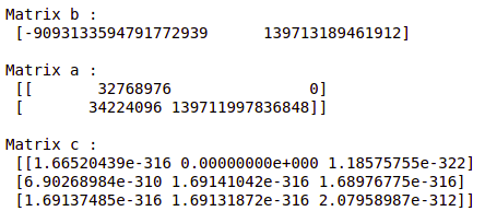
Python3

Matrix b : [0 0] Matrix a : [[0 0] [0 0]] Matrix c : [[0. 0. 0.] [0. 0. 0.] [0. 0. 0.]]

Operations on Numpy Arrays

Arithmetic Operations

Python3

[ 7 77 23 130] [ 7 77 23 130] [ 8 79 26 134] [ 7 77 23 130]

Python3

Python3

[ 10 360 130 3000] [ 10 360 130 3000]

Python3

[ 2.5 14.4 1.3 3.33333333] [ 2.5 14.4 1.3 3.33333333]

NumPy Array Indexing

Indexing can be done in NumPy by using an array as an index. In the case of the slice, a view or shallow copy of the array is returned but in the index array, a copy of the original array is returned. Numpy arrays can be indexed with other arrays or any other sequence with the exception of tuples. The last element is indexed by -1 second last by -2 and so on.

Python NumPy Array Indexing

Python3

A sequential array with a negative step: [10 8 6 4 2] Elements at these indices are: [4 8 6]

NumPy Array Slicing

Consider the syntax x[obj] where x is the array and obj is the index. The slice object is the index in the case of basic slicing. Basic slicing occurs when obj is :

• a slice object that is of the form start: stop: step
• an integer
• or a tuple of slice objects and integers

All arrays generated by basic slicing are always the view in the original array.

Python3

print ( «\n a[10:] gfg-icon gfg-icon_arrow-right-editor padding-2px code-sidebar-button output-icon»>

Array is: [ 0 1 2 3 4 5 6 7 8 9 10 11 12 13 14 15 16 17 18 19] a[-8:17:1] = [12 13 14 15 16] a[10:] = [10 11 12 13 14 15 16 17 18 19]

Ellipsis can also be used along with basic slicing. Ellipsis (…) is the number of : objects needed to make a selection tuple of the same length as the dimensions of the array.

Python3

NumPy Array Broadcasting

The term broadcasting refers to how numpy treats arrays with different Dimensions during arithmetic operations which lead to certain constraints, the smaller array is broadcast across the larger array so that they have compatible shapes.

Let’s assume that we have a large data set, each datum is a list of parameters. In Numpy we have a 2-D array, where each row is a datum and the number of rows is the size of the data set. Suppose we want to apply some sort of scaling to all these data every parameter gets its own scaling factor or say Every parameter is multiplied by some factor.

Just to have a clear understanding, let’s count calories in foods using a macro-nutrient breakdown. Roughly put, the caloric parts of food are made of fats (9 calories per gram), protein (4 CPG), and carbs (4 CPG). So if we list some foods (our data), and for each food list its macro-nutrient breakdown (parameters), we can then multiply each nutrient by its caloric value (apply scaling) to compute the caloric breakdown of every food item.

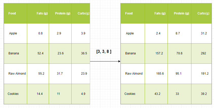
With this transformation, we can now compute all kinds of useful information. For example, what is the total number of calories present in some food or, given a breakdown of my dinner know how many calories did I get from protein and so on.

Let’s see a naive way of producing this computation with Numpy:

Источник