Plot the power spectral density using Matplotlib – Python
matplotlib.pyplot.psd() function is used to plot power spectral density. In the Welch’s average periodogram method for evaluating power spectral density (say, Pxx), the vector ‘x’ is divided equally into NFFT segments. Every segment is windowed by the function window and detrended by the function detrend. The overlap between segments is given by ‘noverlap’. The |fft(i)|*2 of every segment ‘i’ are averaged together to compute P, with buffered scaling to correct for the power loss due to windowing.
Syntax: matplotlib.pyplot.psd(x, NFFT=None, Fs=None, Fc=None, detrend=None, window=None, noverlap=None, pad_to=None, sides=None, scale_by_freq=None, return_line=None, *, data=None, **kwargs)
Parameters:
- x: It is a required parameter of 1D array or a sequence containing data
- Fs: This is a required parameter that has a scalar value and has a default value of 2. Its value is the sampling frequency (samples per time unit). This value is used to calculate Fourier frequencies, freqs, in cycles per unit time.
- window: This is a callable N-D array which is generally a function or a vector of NFFT length. Its default value is window_hanning. When a function is passed as a parameter/argument, it takes a data segment as an argument and returns the windowed version of the segment
- sides: This parameter can have one of the three values namely ‘default’, ‘oneside’ or ‘twoside’. This is used for specifying which sides of the spectrum is to be returned. the ‘default’ gives its default behavior, which returns one-sided for real data and both for complex data. The ‘oneside’ value is used to force return a one-sided spectrum whereas the ‘twoside’ value is to return the two-sided spectrum.
- >pad_to: This parameter holds an integer value tat represents the number of points on which the data segment is padded while performing the FFT. It is important to note that this is different from NFFT, which sets the number of data points used. This can give more points on the plot without increasing the actual resolution of the spectrum (the minimum distance between the resolvable peaks) allowing for more detail. This also corresponds to ‘n’ parameter in the call of fft(). Its default value is None that sets the pad_to equal to NFFT.
- .NFFT: It holds an integer value representing the number of data points used in each block for FFT. The most efficient is the power of 2. Its default value is 256. Using this to get zero paddings must be avoided as it may result in incorrect scaling of the results, instead, pad_to is to be used for the same purpose.
- detrend: It can accept three values namely ‘none’, ‘mean’, ‘linear’ or a callable and has default value as ‘none’.This function is designed to remove the mean or linear trend before fft-ing of each segment. The detrend in Matplotlib is a function unlike the detrend in MATLAB where it is a vector. The ‘detrend_none’, ‘detrend_mean’ and ‘detrend_linear’ are defined by the mlab module, but one can use custom function too. Strings can also choose a function. The ‘none’ calls ‘detrend_none’, the ‘linear’ calls ‘detrend_linear’ and the ‘mean’ calls the ‘detrend_mean’.
- scale_by_freq: It is an optional argument that accepts a boolean value. It is used to specify whether the resulting density should be scaled by scaling the frequency. This would give the density in units of Hz^-1. This makes integration over the returned frequency values. The default for MATLAB compatibility is True.
- noverlap: It is an integer value that represents the total number of points that overlap between segments. The default value for this is 0 suggesting no overlap.
- Fc: It is an integer value representing the offsets of x extent of the plot to reflect the frequency range that is used when a signal is gained and then filtered after which it is downsampled to baseband. the ‘x’ represents the center frequency of x(default value of which is 0)
- return_line: It is a boolean that decides if to include the line objected that is plotted in the return values. This value is False by default
- Pxx: It is a 1-D array which represents the power spectrum P_ before being scaled.
- freqs: It is a !-D array represents the corresponding frequencies to the Pxx elements
- line: It is a Line@D instance which is a line generated by the function. It only returns if return_line is set to True.
Other parameters:
**kwargs the keyword arguments are used to control the Line2D properties
| Property | Description |
|---|---|
| agg_filter | a filter function that takes a (m, n, 3) float array and a dpi value that returns a (m, n, 3) array |
| alpha | float |
| animated | bool |
| antialiased or aa | bool |
| clip_box | Bbox |
| clip_on | bool |
| clip_path | [(Path, Transform)|Patch|None] |
| color or c | color |
| contains | callable |
| dash_capstyle | |
| dash_joinstyle | |
| dashes | sequence of floats(on/off ink in points) or (None, None) |
| drawstyle or ds | , default: ‘default’ |
| figure | figure |
| fillstyle | |
| gid | str |
| in_layout | bool |
| label | object |
| linestyle or lsl | |
| linewidth or lw | float |
| marker | marker style |
| markeredgecolor or mec | color |
| Cmarkeredgewidth or mew | float |
| markerfacecolor or mfc | color |
| markerfacecoloralt or mfcalt | color |
| markersize or ms | float |
| markevery | None or int or (int, int) or slice or List[int] or float or (float, float) |
| path_effects | AbstractPathEffect |
| picker | float or callable[[Artist, Event], Tuple[bool, dict]] |
| pickradius | float |
| rasterized | bool or None |
| sketch_params | (scale: float, length: float, randomness: float) |
| snap | bool or None |
| solid_capstyle | |
| solid_joinstyle | |
| transform | matplotlib.transforms.Transform |
| url | str |
| visible | bool |
| xdata | 1D array |
| ydata | 1D array |
| zorder | float |
scipy.signal.welch#
scipy.signal. welch ( x , fs = 1.0 , window = ‘hann’ , nperseg = None , noverlap = None , nfft = None , detrend = ‘constant’ , return_onesided = True , scaling = ‘density’ , axis = -1 , average = ‘mean’ ) [source] #
Estimate power spectral density using Welch’s method.
Welch’s method [1] computes an estimate of the power spectral density by dividing the data into overlapping segments, computing a modified periodogram for each segment and averaging the periodograms.
Parameters : x array_like
Time series of measurement values
fs float, optional
Sampling frequency of the x time series. Defaults to 1.0.
window str or tuple or array_like, optional
Desired window to use. If window is a string or tuple, it is passed to get_window to generate the window values, which are DFT-even by default. See get_window for a list of windows and required parameters. If window is array_like it will be used directly as the window and its length must be nperseg. Defaults to a Hann window.
nperseg int, optional
Length of each segment. Defaults to None, but if window is str or tuple, is set to 256, and if window is array_like, is set to the length of the window.
noverlap int, optional
Number of points to overlap between segments. If None, noverlap = nperseg // 2 . Defaults to None.
nfft int, optional
Length of the FFT used, if a zero padded FFT is desired. If None, the FFT length is nperseg. Defaults to None.
detrend str or function or False, optional
Specifies how to detrend each segment. If detrend is a string, it is passed as the type argument to the detrend function. If it is a function, it takes a segment and returns a detrended segment. If detrend is False, no detrending is done. Defaults to ‘constant’.
return_onesided bool, optional
If True, return a one-sided spectrum for real data. If False return a two-sided spectrum. Defaults to True, but for complex data, a two-sided spectrum is always returned.
scaling < ‘density’, ‘spectrum’ >, optional
Selects between computing the power spectral density (‘density’) where Pxx has units of V**2/Hz and computing the power spectrum (‘spectrum’) where Pxx has units of V**2, if x is measured in V and fs is measured in Hz. Defaults to ‘density’
axis int, optional
Axis along which the periodogram is computed; the default is over the last axis (i.e. axis=-1 ).
average < ‘mean’, ‘median’ >, optional
Method to use when averaging periodograms. Defaults to ‘mean’.
Array of sample frequencies.
Pxx ndarray
Power spectral density or power spectrum of x.
Simple, optionally modified periodogram
Lomb-Scargle periodogram for unevenly sampled data
An appropriate amount of overlap will depend on the choice of window and on your requirements. For the default Hann window an overlap of 50% is a reasonable trade off between accurately estimating the signal power, while not over counting any of the data. Narrower windows may require a larger overlap.
If noverlap is 0, this method is equivalent to Bartlett’s method [2].
P. Welch, “The use of the fast Fourier transform for the estimation of power spectra: A method based on time averaging over short, modified periodograms”, IEEE Trans. Audio Electroacoust. vol. 15, pp. 70-73, 1967.
M.S. Bartlett, “Periodogram Analysis and Continuous Spectra”, Biometrika, vol. 37, pp. 1-16, 1950.
>>> import numpy as np >>> from scipy import signal >>> import matplotlib.pyplot as plt >>> rng = np.random.default_rng()
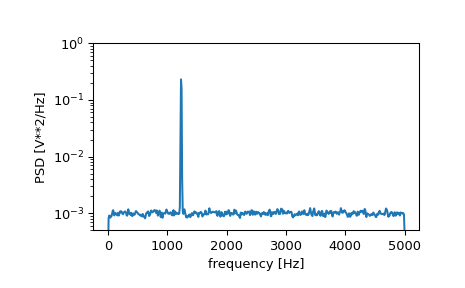
Generate a test signal, a 2 Vrms sine wave at 1234 Hz, corrupted by 0.001 V**2/Hz of white noise sampled at 10 kHz.
>>> fs = 10e3 >>> N = 1e5 >>> amp = 2*np.sqrt(2) >>> freq = 1234.0 >>> noise_power = 0.001 * fs / 2 >>> time = np.arange(N) / fs >>> x = amp*np.sin(2*np.pi*freq*time) >>> x += rng.normal(scale=np.sqrt(noise_power), size=time.shape)
Compute and plot the power spectral density.
>>> f, Pxx_den = signal.welch(x, fs, nperseg=1024) >>> plt.semilogy(f, Pxx_den) >>> plt.ylim([0.5e-3, 1]) >>> plt.xlabel('frequency [Hz]') >>> plt.ylabel('PSD [V**2/Hz]') >>> plt.show()
If we average the last half of the spectral density, to exclude the peak, we can recover the noise power on the signal.
>>> np.mean(Pxx_den[256:]) 0.0009924865443739191
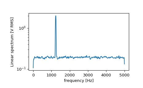
Now compute and plot the power spectrum.
>>> f, Pxx_spec = signal.welch(x, fs, 'flattop', 1024, scaling='spectrum') >>> plt.figure() >>> plt.semilogy(f, np.sqrt(Pxx_spec)) >>> plt.xlabel('frequency [Hz]') >>> plt.ylabel('Linear spectrum [V RMS]') >>> plt.show()
The peak height in the power spectrum is an estimate of the RMS amplitude.
>>> np.sqrt(Pxx_spec.max()) 2.0077340678640727
If we now introduce a discontinuity in the signal, by increasing the amplitude of a small portion of the signal by 50, we can see the corruption of the mean average power spectral density, but using a median average better estimates the normal behaviour.
>>> x[int(N//2):int(N//2)+10] *= 50. >>> f, Pxx_den = signal.welch(x, fs, nperseg=1024) >>> f_med, Pxx_den_med = signal.welch(x, fs, nperseg=1024, average='median') >>> plt.semilogy(f, Pxx_den, label='mean') >>> plt.semilogy(f_med, Pxx_den_med, label='median') >>> plt.ylim([0.5e-3, 1]) >>> plt.xlabel('frequency [Hz]') >>> plt.ylabel('PSD [V**2/Hz]') >>> plt.legend() >>> plt.show()

