Получение обратной матрицы python

Linear algebra ( numpy.linalg )#

The NumPy linear algebra functions rely on BLAS and LAPACK to provide efficient low level implementations of standard linear algebra algorithms. Those libraries may be provided by NumPy itself using C versions of a subset of their reference implementations but, when possible, highly optimized libraries that take advantage of specialized processor functionality are preferred. Examples of such libraries are OpenBLAS, MKL (TM), and ATLAS. Because those libraries are multithreaded and processor dependent, environmental variables and external packages such as threadpoolctl may be needed to control the number of threads or specify the processor architecture.

The SciPy library also contains a linalg submodule, and there is overlap in the functionality provided by the SciPy and NumPy submodules. SciPy contains functions not found in numpy.linalg , such as functions related to LU decomposition and the Schur decomposition, multiple ways of calculating the pseudoinverse, and matrix transcendentals such as the matrix logarithm. Some functions that exist in both have augmented functionality in scipy.linalg . For example, scipy.linalg.eig can take a second matrix argument for solving generalized eigenvalue problems. Some functions in NumPy, however, have more flexible broadcasting options. For example, numpy.linalg.solve can handle “stacked” arrays, while scipy.linalg.solve accepts only a single square array as its first argument.

The term matrix as it is used on this page indicates a 2d numpy.array object, and not a numpy.matrix object. The latter is no longer recommended, even for linear algebra. See the matrix object documentation for more information.

The @ operator#

Introduced in NumPy 1.10.0, the @ operator is preferable to other methods when computing the matrix product between 2d arrays. The numpy.matmul function implements the @ operator.

Matrix and vector products#

Dot product of two arrays.

Compute the dot product of two or more arrays in a single function call, while automatically selecting the fastest evaluation order.

Return the dot product of two vectors.

Inner product of two arrays.

Compute the outer product of two vectors.

Matrix product of two arrays.

Compute tensor dot product along specified axes.

einsum (subscripts, *operands[, out, dtype, . ])

Evaluates the Einstein summation convention on the operands.

einsum_path (subscripts, *operands[, optimize])

Evaluates the lowest cost contraction order for an einsum expression by considering the creation of intermediate arrays.

Raise a square matrix to the (integer) power n.

Kronecker product of two arrays.

Decompositions#

Compute the qr factorization of a matrix.

linalg.svd (a[, full_matrices, compute_uv, . ])

Singular Value Decomposition.

Matrix eigenvalues#

Compute the eigenvalues and right eigenvectors of a square array.

Return the eigenvalues and eigenvectors of a complex Hermitian (conjugate symmetric) or a real symmetric matrix.

Compute the eigenvalues of a general matrix.

Compute the eigenvalues of a complex Hermitian or real symmetric matrix.

Norms and other numbers#

Compute the condition number of a matrix.

Compute the determinant of an array.

Return matrix rank of array using SVD method

Compute the sign and (natural) logarithm of the determinant of an array.

trace (a[, offset, axis1, axis2, dtype, out])

Return the sum along diagonals of the array.

Solving equations and inverting matrices#

Solve a linear matrix equation, or system of linear scalar equations.

Solve the tensor equation a x = b for x.

Return the least-squares solution to a linear matrix equation.

Compute the (multiplicative) inverse of a matrix.

Compute the (Moore-Penrose) pseudo-inverse of a matrix.

Compute the ‘inverse’ of an N-dimensional array.

Exceptions#

Generic Python-exception-derived object raised by linalg functions.

Linear algebra on several matrices at once#

Several of the linear algebra routines listed above are able to compute results for several matrices at once, if they are stacked into the same array.

This is indicated in the documentation via input parameter specifications such as a : (. M, M) array_like . This means that if for instance given an input array a.shape == (N, M, M) , it is interpreted as a “stack” of N matrices, each of size M-by-M. Similar specification applies to return values, for instance the determinant has det : (. ) and will in this case return an array of shape det(a).shape == (N,) . This generalizes to linear algebra operations on higher-dimensional arrays: the last 1 or 2 dimensions of a multidimensional array are interpreted as vectors or matrices, as appropriate for each operation.

Источник

numpy.linalg.inv#

Given a square matrix a, return the matrix ainv satisfying dot(a, ainv) = dot(ainv, a) = eye(a.shape[0]) .

Parameters : a (…, M, M) array_like

Returns : ainv (…, M, M) ndarray or matrix

(Multiplicative) inverse of the matrix a.

If a is not square or inversion fails.

Similar function in SciPy.

Broadcasting rules apply, see the numpy.linalg documentation for details.

>>> from numpy.linalg import inv >>> a = np.array([[1., 2.], [3., 4.]]) >>> ainv = inv(a) >>> np.allclose(np.dot(a, ainv), np.eye(2)) True >>> np.allclose(np.dot(ainv, a), np.eye(2)) True 

If a is a matrix object, then the return value is a matrix as well:

>>> ainv = inv(np.matrix(a)) >>> ainv matrix([[-2. , 1. ], [ 1.5, -0.5]]) 

Inverses of several matrices can be computed at once:

>>> a = np.array([[[1., 2.], [3., 4.]], [[1, 3], [3, 5]]]) >>> inv(a) array([[[-2. , 1. ], [ 1.5 , -0.5 ]], [[-1.25, 0.75], [ 0.75, -0.25]]]) 

Источник

Линейная алгебра на Python. [Урок 5]. Обратная матрица и ранг матрицы

Обратной матрицей A -1 матрицы A называют матрицу, удовлетворяющую следующему равенству:

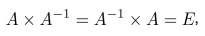
где – E это единичная матрица.

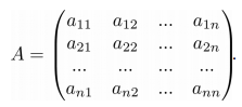
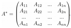
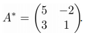
Для того, чтобы у квадратной матрицы A была обратная матрица необходимо и достаточно чтобы определитель |A| был не равен нулю. Введем понятие союзной матрицы . Союзная матрица A* строится на базе исходной A путем замены всех элементов матрицы A на их алгебраические дополнения.

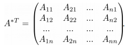
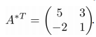
Транспонируя матрицу A*, мы получим так называемую присоединенную матрицу A* T :

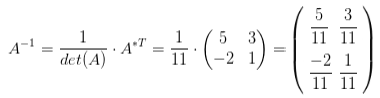
Теперь, зная как вычислять определитель и присоединенную матрицу, мы можем определить матрицу A -1 , обратную матрице A:

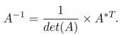
Пример вычисления обратной матрицы. Пусть дана исходная матрица A, следующего вида:

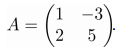
Для начала найдем определитель матрицы A:

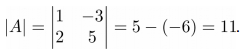
Как видно из приведенных вычислений, определитель матрицы не равен нулю, значит у матрицы A есть обратная. Построим присоединенную матрицу, для этого вычислим алгебраические дополнения для каждого элемента матрицы A:

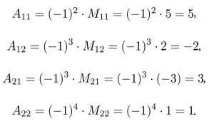
Союзная матрица будет иметь следующий вид:

Присоединенная матрица получается из союзной путем транспонирования:

Решим задачу определения обратной матрицы на Python. Для получения обратной матрицы будем использовать функцию inv():

>>> A = np.matrix('1 -3; 2 5') >>> A_inv = np.linalg.inv(A) >>> print(A_inv) [[ 0.45454545 0.27272727] [-0.18181818 0.09090909]]

Рассмотрим свойства обратной матрицы.

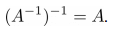
Свойство 1 . Обратная матрица обратной матрицы есть исходная матрица:

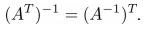
>>> A = np.matrix('1. -3.; 2. 5.') >>> A_inv = np.linalg.inv(A) >>> A_inv_inv = np.linalg.inv(A_inv) >>> print(A) [[1. -3.] [2. 5.]] >>> print(A_inv_inv) [[1. -3.] [2. 5.]]

Свойство 2 . Обратная матрица транспонированной матрицы равна транспонированной матрице от обратной матрицы:

>>> A = np.matrix('1. -3.; 2. 5.') >>> L = np.linalg.inv(A.T) >>> R = (np.linalg.inv(A)).T >>> print(L) [[ 0.45454545 -0.18181818] [ 0.27272727 0.09090909]] >>> print(R) [[ 0.45454545 -0.18181818] [ 0.27272727 0.09090909]]

Свойство 3 . Обратная матрица произведения матриц равна произведению обратных матриц:

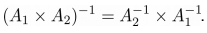
>>> A = np.matrix('1. -3.; 2. 5.') >>> B = np.matrix('7. 6.; 1. 8.') >>> L = np.linalg.inv(A.dot(B)) >>> R = np.linalg.inv(B).dot(np.linalg.inv(A)) >>> print(L) [[ 0.09454545 0.03272727] [-0.03454545 0.00727273]] >>> print(R) [[ 0.09454545 0.03272727] [-0.03454545 0.00727273]]

Ранг матрицы

Ранг матрицы является еще одной важной численной характеристикой. Рангом называют максимальное число линейно независимых строк (столбцов) матрицы. Линейная независимость означает, что строки (столбцы) не могут быть линейно выражены через другие строки (столбцы). Ранг матрицы можно найти через ее миноры, он равен наибольшему порядку минора, который не равен нулю. Существование ранга у матрицы не зависит от того квадратная она или нет.

Вычислим ранг матрицы с помощью Python. Создадим единичную матрицу:

>>> m_eye = np.eye(4) >>> print(m_eye) [[1. 0. 0. 0.] [0. 1. 0. 0.] [0. 0. 1. 0.] [0. 0. 0. 1.]]

Ранг такой матрицы равен количеству ее столбцов (или строк), в нашем случае ранг будет равен четырем, для его вычисления на Python воспользуемся функцией matrix_rank():

>>> rank = np.linalg.matrix_rank(m_eye) >>> print(rank) 4

Если мы приравняем элемент в нижнем правом углу к нулю, то ранг станет равен трем:

>>> m_eye[3][3] = 0 >>> print(m_eye) [[1. 0. 0. 0.] [0. 1. 0. 0.] [0. 0. 1. 0.] [0. 0. 0. 0.]] >>> rank = np.linalg.matrix_rank(m_eye) >>> print(rank) 3

P.S.

Вводные уроки по “Линейной алгебре на Python” вы можете найти соответствующей странице нашего сайта . Все уроки по этой теме собраны в книге “Линейная алгебра на Python”.

Если вам интересна тема анализа данных, то мы рекомендуем ознакомиться с библиотекой Pandas. Для начала вы можете познакомиться с вводными уроками. Все уроки по библиотеке Pandas собраны в книге “Pandas. Работа с данными”.

Линейная алгебра на Python. [Урок 5]. Обратная матрица и ранг матрицы : 1 комментарий

1. pedro kekulé 23.10.2019 i want that help me
   1) написать программу вычисляющую обратную матрицу 2) написать программу для решения СЛАУ с помощью обратной матрицы 3) сравнить скорость работы всех трёх методов решения СЛАУ

Источник