Matplotlib legend
Matplotlib has native support for legends. Legends can be placed in various positions: A legend can be placed inside or outside the chart and the position can be moved.
The legend() method adds the legend to the plot. In this article we will show you some examples of legends using matplotlib.
Related course
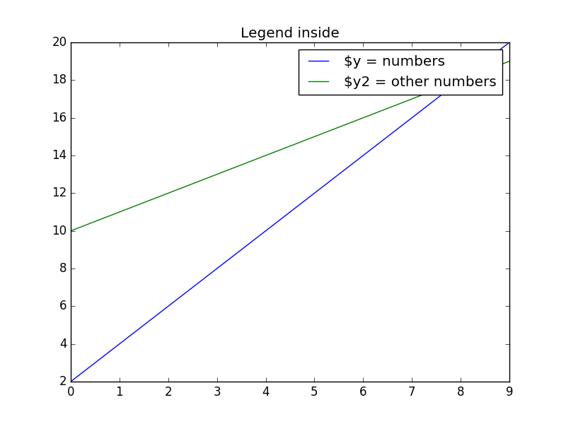
Matplotlib legend inside
To place the legend inside, simply call legend():
import matplotlib.pyplot as plt
import numpy as np
y = [2,4,6,8,10,12,14,16,18,20]
y2 = [10,11,12,13,14,15,16,17,18,19]
x = np.arange(10)
fig = plt.figure()
ax = plt.subplot(111)
ax.plot(x, y, label=‘$y = numbers’)
ax.plot(x, y2, label=‘$y2 = other numbers’)
plt.title(‘Legend inside’)
ax.legend()
plt.show()
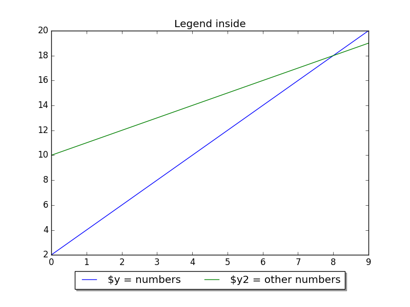
Matplotlib legend on bottom
To place the legend on the bottom, change the legend() call to:
ax.legend(loc=‘upper center’, bbox_to_anchor=(0.5, —0.05), shadow=True, ncol=2)
Take into account that we set the number of columns two ncol=2 and set a shadow.
The complete code would be:
import matplotlib.pyplot as plt
import numpy as np
y = [2,4,6,8,10,12,14,16,18,20]
y2 = [10,11,12,13,14,15,16,17,18,19]
x = np.arange(10)
fig = plt.figure()
ax = plt.subplot(111)
ax.plot(x, y, label=‘$y = numbers’)
ax.plot(x, y2, label=‘$y2 = other numbers’)
plt.title(‘Legend inside’)
ax.legend(loc=‘upper center’, bbox_to_anchor=(0.5, —0.05), shadow=True, ncol=2)
plt.show()
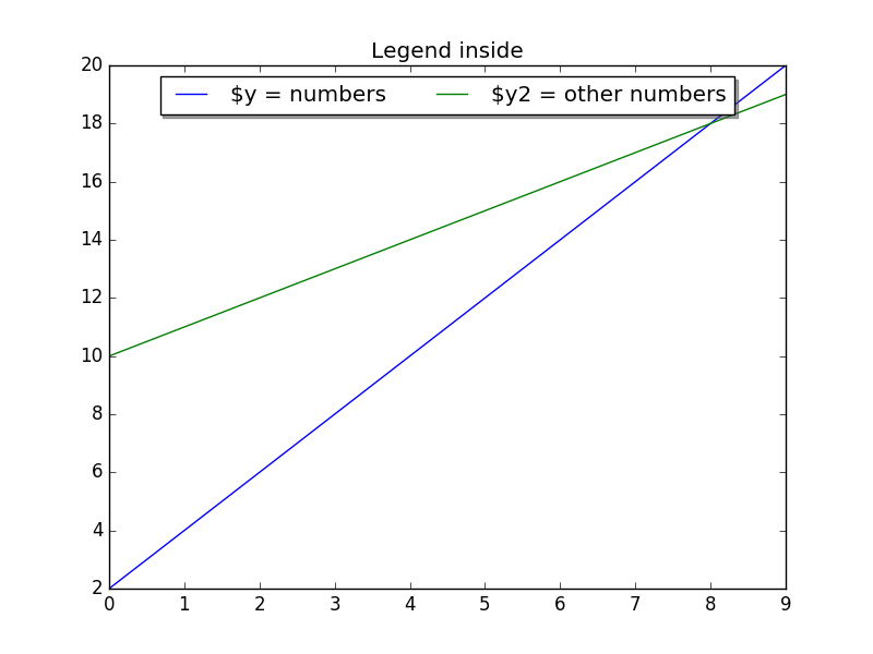
Matplotlib legend on top
To put the legend on top, change the bbox_to_anchor values:
ax.legend(loc=‘upper center’, bbox_to_anchor=(0.5, 1.00), shadow=True, ncol=2)
import matplotlib.pyplot as plt
import numpy as np
y = [2,4,6,8,10,12,14,16,18,20]
y2 = [10,11,12,13,14,15,16,17,18,19]
x = np.arange(10)
fig = plt.figure()
ax = plt.subplot(111)
ax.plot(x, y, label=‘$y = numbers’)
ax.plot(x, y2, label=‘$y2 = other numbers’)
plt.title(‘Legend inside’)
ax.legend(loc=‘upper center’, bbox_to_anchor=(0.5, 1.00), shadow=True, ncol=2)
plt.show()
Legend outside right
We can put the legend ouside by resizing the box and puting the legend relative to that:
chartBox = ax.get_position()
ax.set_position([chartBox.x0, chartBox.y0, chartBox.width*0.6, chartBox.height])
ax.legend(loc=‘upper center’, bbox_to_anchor=(1.45, 0.8), shadow=True, ncol=1)
import matplotlib.pyplot as plt
import numpy as np
y = [2,4,6,8,10,12,14,16,18,20]
y2 = [10,11,12,13,14,15,16,17,18,19]
x = np.arange(10)
fig = plt.figure()
ax = plt.subplot(111)
ax.plot(x, y, label=‘$y = numbers’)
ax.plot(x, y2, label=‘$y2 = other numbers’)
plt.title(‘Legend outside’)
chartBox = ax.get_position()
ax.set_position([chartBox.x0, chartBox.y0, chartBox.width*0.6, chartBox.height])
ax.legend(loc=‘upper center’, bbox_to_anchor=(1.45, 0.8), shadow=True, ncol=1)
plt.show()
Matplotlib. Урок 3.1. Настройка графиков. Работа с легендой


Следующие несколько уроков будут посвящены настройке графиков. Начнем с работы с легендой. В данном уроке будут рассмотрены следующие темы: отображение легенды, настройка ее расположения на графике, дополнительные параметры для более тонкой настройки ее внешнего вида.
Отображение легенды
Для отображения легенды на графике используется функция legend() , возможны следующие варианты ее вызова:
legend() legend(labels) legend(handles, labels)
В первом варианте в качестве меток для легенды будет использоваться метки, указанные в функциях построения графиков (параметр label ):
x = [1, 5, 10, 15, 20] y1 = [1, 7, 3, 5, 11] y2 = [4, 3, 1, 8, 12] plt.plot(x, y1, 'o-r', label='line 1') plt.plot(x, y2, 'o-.g', label='line 2') plt.legend()

Второй вариант позволят самостоятельно указать текстовую метку для отображаемых данных:
plt.plot(x, y1, 'o-r') plt.plot(x, y2, 'o-.g') plt.legend(['L1', 'L2'])

В третьем варианте можно вручную указать соответствие линии и меток для них:
line1, = plt.plot(x, y1, 'o-b') line2, = plt.plot(x, y2, 'o-.m') plt.legend((line2, line1), ['L2', 'L1'])

Расположение легенды на графике
Место расположения легенды определяется параметром loc , которое может принимать одно из следующих значений:
| Строковое описание | Код |
| ‘best’ | 0 |
| ‘upper right’ | 1 |
| ‘upper left’ | 2 |
| ‘lower left’ | 3 |
| ‘lower right’ | 4 |
| ‘right’ | 5 |
| ‘center left’ | 6 |
| ‘center right’ | 7 |
| ‘lower center’ | 8 |
| ‘upper center’ | 9 |
| ‘center’ | 10 |
| ‘upper right’ | 0 |
Ниже представлен пример, реализующий различные варианты расстановки легенды через параметр loc :
locs = ['best', 'upper right', 'upper left', 'lower left', 'lower right', 'right', 'center left', 'center right', 'lower center', 'upper center', 'center'] plt.figure(figsize=(12, 12)) for i in range(3): for j in range(4): if i*4+j < 11: plt.subplot(3, 4, i*4+j+1) plt.title(locs[i*4+j]) plt.plot(x, y1, 'o-r', label='line 1') plt.plot(x, y2, 'o-.g', label='line 2') plt.legend(loc=locs[i*4+j]) else: break

Для более гибкого управление положением объекта можно воспользоваться параметром bbox_to_anchor функции legend() . Этому параметру присваивается кортеж, состоящий из четырех или двух элементов:
bbox_to_anchor = (x, y, width, height) bbox_to_anchor = (x, y)
Пример использования параметра bbox_to_anchor :
plt.plot(x, y1, 'o-r', label='line 1') plt.plot(x, y2, 'o-.g', label='line 2') plt.legend(bbox_to_anchor=(1, 0.6))

Дополнительные параметры настройки отображения легенды
В таблице ниже представлены дополнительные параметры, которые можно использовать для более тонкой настройки легенды.
| Параметр | Тип | Описание |
| fontsize | int или float или | Размера шрифта надписи легенды |
| frameon | bool | Отображение рамки легенды |
| framealpha | None или float | Прозрачность легенды |
| facecolor | None или str | Цвет заливки |
| edgecolor | None или str | Цвет рамки |
| title | None или str | Текст заголовка |
| title_fontsize | None или str | Размер шрифта |
Пример работы с параметрами:
plt.plot(x, y1, 'o-r', label='line 1') plt.plot(x, y2, 'o-.g', label='line 2') plt.legend(fontsize=14, shadow=True, framealpha=1, facecolor='y', edgecolor='r', title='Легенда')

Дополнительные материалы
Дополнительную информацию по работе с легендой можете найти в следующих официальных материалах проекта Matplotlib:
P.S.
Вводные уроки по “Линейной алгебре на Python” вы можете найти соответствующей странице нашего сайта . Все уроки по этой теме собраны в книге “Линейная алгебра на Python”.
Если вам интересна тема анализа данных, то мы рекомендуем ознакомиться с библиотекой Pandas. Для начала вы можете познакомиться с вводными уроками. Все уроки по библиотеке Pandas собраны в книге “Pandas. Работа с данными”.