1.4. Support Vector Machines
Support vector machines (SVMs) are a set of supervised learning methods used for classification , regression and outliers detection .
The advantages of support vector machines are:
- Effective in high dimensional spaces.
- Still effective in cases where number of dimensions is greater than the number of samples.
- Uses a subset of training points in the decision function (called support vectors), so it is also memory efficient.
- Versatile: different Kernel functions can be specified for the decision function. Common kernels are provided, but it is also possible to specify custom kernels.
The disadvantages of support vector machines include:
- If the number of features is much greater than the number of samples, avoid over-fitting in choosing Kernel functions and regularization term is crucial.
- SVMs do not directly provide probability estimates, these are calculated using an expensive five-fold cross-validation (see Scores and probabilities , below).
The support vector machines in scikit-learn support both dense ( numpy.ndarray and convertible to that by numpy.asarray ) and sparse (any scipy.sparse ) sample vectors as input. However, to use an SVM to make predictions for sparse data, it must have been fit on such data. For optimal performance, use C-ordered numpy.ndarray (dense) or scipy.sparse.csr_matrix (sparse) with dtype=float64 .
1.4.1. Classification
SVC , NuSVC and LinearSVC are classes capable of performing binary and multi-class classification on a dataset.
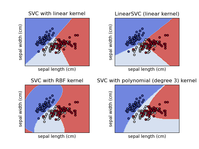
SVC and NuSVC are similar methods, but accept slightly different sets of parameters and have different mathematical formulations (see section Mathematical formulation ). On the other hand, LinearSVC is another (faster) implementation of Support Vector Classification for the case of a linear kernel. Note that LinearSVC does not accept parameter kernel , as this is assumed to be linear. It also lacks some of the attributes of SVC and NuSVC , like support_ .
As other classifiers, SVC , NuSVC and LinearSVC take as input two arrays: an array X of shape (n_samples, n_features) holding the training samples, and an array y of class labels (strings or integers), of shape (n_samples) :
>>> from sklearn import svm >>> X = [[0, 0], [1, 1]] >>> y = [0, 1] >>> clf = svm.SVC() >>> clf.fit(X, y) SVC()
After being fitted, the model can then be used to predict new values:
SVMs decision function (detailed in the Mathematical formulation ) depends on some subset of the training data, called the support vectors. Some properties of these support vectors can be found in attributes support_vectors_ , support_ and n_support_ :
>>> # get support vectors >>> clf.support_vectors_ array([[0., 0.], [1., 1.]]) >>> # get indices of support vectors >>> clf.support_ array([0, 1]. ) >>> # get number of support vectors for each class >>> clf.n_support_ array([1, 1]. )
1.4.1.1. Multi-class classification
SVC and NuSVC implement the “one-versus-one” approach for multi-class classification. In total, n_classes * (n_classes — 1) / 2 classifiers are constructed and each one trains data from two classes. To provide a consistent interface with other classifiers, the decision_function_shape option allows to monotonically transform the results of the “one-versus-one” classifiers to a “one-vs-rest” decision function of shape (n_samples, n_classes) .
>>> X = [[0], [1], [2], [3]] >>> Y = [0, 1, 2, 3] >>> clf = svm.SVC(decision_function_shape='ovo') >>> clf.fit(X, Y) SVC(decision_function_shape='ovo') >>> dec = clf.decision_function([[1]]) >>> dec.shape[1] # 4 classes: 4*3/2 = 6 6 >>> clf.decision_function_shape = "ovr" >>> dec = clf.decision_function([[1]]) >>> dec.shape[1] # 4 classes 4
On the other hand, LinearSVC implements “one-vs-the-rest” multi-class strategy, thus training n_classes models.
>>> lin_clf = svm.LinearSVC(dual="auto") >>> lin_clf.fit(X, Y) LinearSVC(dual='auto') >>> dec = lin_clf.decision_function([[1]]) >>> dec.shape[1] 4
See Mathematical formulation for a complete description of the decision function.
Details on multi-class strategies Click for more details
Note that the LinearSVC also implements an alternative multi-class strategy, the so-called multi-class SVM formulated by Crammer and Singer [ 16 ] , by using the option multi_class=’crammer_singer’ . In practice, one-vs-rest classification is usually preferred, since the results are mostly similar, but the runtime is significantly less.
For “one-vs-rest” LinearSVC the attributes coef_ and intercept_ have the shape (n_classes, n_features) and (n_classes,) respectively. Each row of the coefficients corresponds to one of the n_classes “one-vs-rest” classifiers and similar for the intercepts, in the order of the “one” class.
In the case of “one-vs-one” SVC and NuSVC , the layout of the attributes is a little more involved. In the case of a linear kernel, the attributes coef_ and intercept_ have the shape (n_classes * (n_classes — 1) / 2, n_features) and (n_classes * (n_classes — 1) / 2) respectively. This is similar to the layout for LinearSVC described above, with each row now corresponding to a binary classifier. The order for classes 0 to n is “0 vs 1”, “0 vs 2” , … “0 vs n”, “1 vs 2”, “1 vs 3”, “1 vs n”, . . . “n-1 vs n”.
The shape of dual_coef_ is (n_classes-1, n_SV) with a somewhat hard to grasp layout. The columns correspond to the support vectors involved in any of the n_classes * (n_classes — 1) / 2 “one-vs-one” classifiers. Each support vector v has a dual coefficient in each of the n_classes — 1 classifiers comparing the class of v against another class. Note that some, but not all, of these dual coefficients, may be zero. The n_classes — 1 entries in each column are these dual coefficients, ordered by the opposing class.
This might be clearer with an example: consider a three class problem with class 0 having three support vectors \(v^_0, v^_0, v^_0\) and class 1 and 2 having two support vectors \(v^_1, v^_1\) and \(v^_2, v^_2\) respectively. For each support vector \(v^_i\) , there are two dual coefficients. Let’s call the coefficient of support vector \(v^_i\) in the classifier between classes \(i\) and \(k\) \(\alpha^_\) . Then dual_coef_ looks like this:
DataTechNotes
We’ll create a random sample dataset for this tutorial by using the make_blob() function. We’ll check the dataset by visualizing it in a plot.
random.seed(13) x, _ = make_blobs(n_samples=200, centers=1, cluster_std=.3, center_box=(8, 8)) plt.scatter(x[:,0], x[:,1]) plt.show() 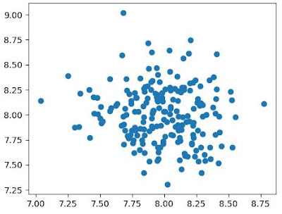
Defining the model and prediction
We’ll define the model by using the OneClassSVM class of Scikit-learn API. Here, we’ll set RBF for kernel type and define the gamma and the ‘nu’ arguments.
svm = OneClassSVM(kernel='rbf', gamma=0.001, nu=0.03) print(svm) OneClassSVM(cache_size=200, coef0=0.0, degree=3, gamma=0.001, kernel='rbf', max_iter=-1, nu=0.03, shrinking=True, tol=0.001, verbose=False) We’ll fit the model with x dataset and get the prediction data by using the fit() and predict() method.
svm.fit(x) pred = svm.predict(x) Next, we’ll extract the negative outputs as the outliers.
anom_index = where(pred==-1) values = x[anom_index] Finally, we’ll visualize the results in a plot by highlighting the anomalies with a color.
plt.scatter(x[:,0], x[:,1]) plt.scatter(values[:,0], values[:,1], color='r') plt.show() 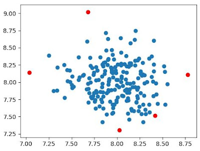
Anomaly detection with scores
We can find anomalies by using their scores. In this method, we’ll define the model, fit it on the x data by using the fit_predict() method. We’ll calculate the outliers according to the score value of each element.
svm = OneClassSVM(kernel='rbf', gamma=0.001, nu=0.02) print(svm) Next, we’ll fit the model on x dataset, then extract the samples score.
pred = svm.fit_predict(x) scores = svm.score_samples(x) Next, we’ll obtain the threshold value from the scores by using the quantile function. Here, we’ll get the lowest 3 percent of score values as the anomalies.
thresh = quantile(scores, 0.03) print(thresh) Next, we’ll extract the anomalies by comparing the threshold value and identify the values of elements.
index = where(scoresthresh) values = x[index] Finally, we can visualize the results in a plot by highlighting the anomalies with a color.
plt.scatter(x[:,0], x[:,1]) plt.scatter(values[:,0], values[:,1], color='r') plt.show() 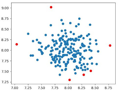
In this tutorial, we’ve learned how to detect the anomalies with the One-class SVM method by using the Scikit-learn’s OneClassSVM class in Python. We’ve seen two types of outlier detection methods with OneClassSVM. The full source code is listed below.
from sklearn.svm import OneClassSVM from sklearn.datasets import make_blobs from numpy import quantile, where, random import matplotlib.pyplot as plt random.seed(13) x, _ = make_blobs(n_samples=200, centers=1, cluster_std=.3, center_box=(8, 8)) plt.scatter(x[:,0], x[:,1]) plt.show() svm = OneClassSVM(kernel='rbf', gamma=0.001, nu=0.03) print(svm) svm.fit(x) pred = svm.predict(x) anom_index = where(pred==-1) values = x[anom_index] plt.scatter(x[:,0], x[:,1]) plt.scatter(values[:,0], values[:,1], color='r') plt.show() svm = OneClassSVM(kernel='rbf', gamma=0.001, nu=0.02) print(svm) pred = svm.fit_predict(x) scores = svm.score_samples(x) thresh = quantile(scores, 0.03) print(thresh) index = where(scoresthresh) values = x[index] plt.scatter(x[:,0], x[:,1]) plt.scatter(values[:,0], values[:,1], color='r') plt.show()
One-class SVM with non-linear kernel (RBF)
An example using a one-class SVM for novelty detection.
One-class SVM is an unsupervised algorithm that learns a decision function for novelty detection: classifying new data as similar or different to the training set.
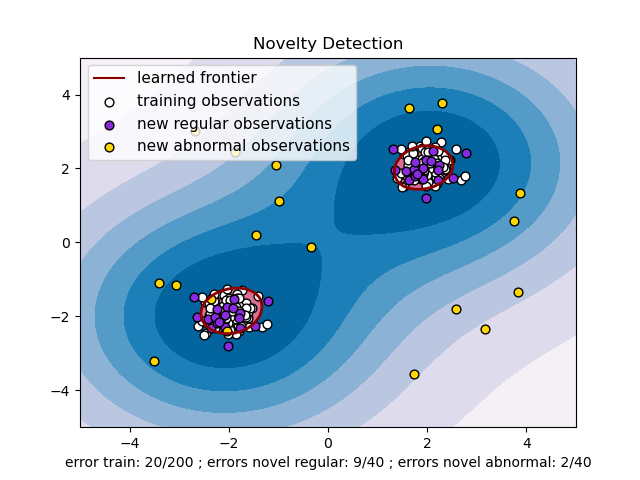
import matplotlib.font_manager import matplotlib.pyplot as plt import numpy as np from sklearn import svm xx, yy = np.meshgrid(np.linspace(-5, 5, 500), np.linspace(-5, 5, 500)) # Generate train data X = 0.3 * np.random.randn(100, 2) X_train = np.r_[X + 2, X - 2] # Generate some regular novel observations X = 0.3 * np.random.randn(20, 2) X_test = np.r_[X + 2, X - 2] # Generate some abnormal novel observations X_outliers = np.random.uniform(low=-4, high=4, size=(20, 2)) # fit the model clf = svm.OneClassSVM(nu=0.1, kernel="rbf", gamma=0.1) clf.fit(X_train) y_pred_train = clf.predict(X_train) y_pred_test = clf.predict(X_test) y_pred_outliers = clf.predict(X_outliers) n_error_train = y_pred_train[y_pred_train == -1].size n_error_test = y_pred_test[y_pred_test == -1].size n_error_outliers = y_pred_outliers[y_pred_outliers == 1].size # plot the line, the points, and the nearest vectors to the plane Z = clf.decision_function(np.c_[xx.ravel(), yy.ravel()]) Z = Z.reshape(xx.shape) plt.title("Novelty Detection") plt.contourf(xx, yy, Z, levels=np.linspace(Z.min(), 0, 7), cmap=plt.cm.PuBu) a = plt.contour(xx, yy, Z, levels=[0], linewidths=2, colors="darkred") plt.contourf(xx, yy, Z, levels=[0, Z.max()], colors="palevioletred") s = 40 b1 = plt.scatter(X_train[:, 0], X_train[:, 1], c="white", s=s, edgecolors="k") b2 = plt.scatter(X_test[:, 0], X_test[:, 1], c="blueviolet", s=s, edgecolors="k") c = plt.scatter(X_outliers[:, 0], X_outliers[:, 1], c="gold", s=s, edgecolors="k") plt.axis("tight") plt.xlim((-5, 5)) plt.ylim((-5, 5)) plt.legend( [a.collections[0], b1, b2, c], [ "learned frontier", "training observations", "new regular observations", "new abnormal observations", ], loc="upper left", prop=matplotlib.font_manager.FontProperties(size=11), ) plt.xlabel( "error train: %d/200 ; errors novel regular: %d/40 ; errors novel abnormal: %d/40" % (n_error_train, n_error_test, n_error_outliers) ) plt.show()
Total running time of the script: ( 0 minutes 0.405 seconds)