Обход в глубину питон

Depth-First Search and Breadth-First Search in Python

Graph theory and in particular the graph ADT (abstract data-type) is widely explored and implemented in the field of Computer Science and Mathematics. Consisting of vertices (nodes) and the edges (optionally directed/weighted) that connect them, the data-structure is effectively able to represent and solve many problem domains. One of the most popular areas of algorithm design within this space is the problem of checking for the existence or (shortest) path between two or more vertices in the graph. Properties such as edge weighting and direction are two such factors that the algorithm designer can take into consideration. In this post I will be exploring two of the simpler available algorithms, Depth-First and Breath-First search to achieve the goals highlighted below:

• Find all vertices in a subject vertices connected component.
• Return all available paths between two vertices.
• And in the case of BFS, return the shortest path (length measured by number of path edges).

The Graph

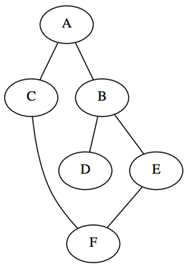
So as to clearly discuss each algorithm I have crafted a connected graph with six vertices and six incident edges. The resulting graph is undirected with no assigned edge weightings, as length will be evaluated based on the number of path edges traversed. There are two popular options for representing a graph, the first being an adjacency matrix (effective with dense graphs) and second an adjacency list (effective with sparse graphs). I have opted to implement an adjacency list which stores each node in a dictionary along with a set containing their adjacent nodes. As the graph is undirected each edge is stored in both incident nodes adjacent sets.

graph = 'A': set(['B', 'C']), 'B': set(['A', 'D', 'E']), 'C': set(['A', 'F']), 'D': set(['B']), 'E': set(['B', 'F']), 'F': set(['C', 'E'])> 

Looking at the graph depiction below you will also notice the inclusion of a cycle, by the adjacent connections between ‘F’ and ‘C/E’. This has been purposely included to provide the algorithms with the option to return multiple paths between two desired nodes.

Depth-First Search

The first algorithm I will be discussing is Depth-First search which as the name hints at, explores possible vertices (from a supplied root) down each branch before backtracking. This property allows the algorithm to be implemented succinctly in both iterative and recursive forms. Below is a listing of the actions performed upon each visit to a node.

• Mark the current vertex as being visited.
• Explore each adjacent vertex that is not included in the visited set.

Connected Component

The implementation below uses the stack data-structure to build-up and return a set of vertices that are accessible within the subjects connected component. Using Python’s overloading of the subtraction operator to remove items from a set, we are able to add only the unvisited adjacent vertices.

def dfs(graph, start): visited, stack = set(), [start] while stack: vertex = stack.pop() if vertex not in visited: visited.add(vertex) stack.extend(graph[vertex] - visited) return visited dfs(graph, 'A') # 

The second implementation provides the same functionality as the first, however, this time we are using the more succinct recursive form. Due to a common Python gotcha with default parameter values being created only once, we are required to create a new visited set on each user invocation. Another Python language detail is that function variables are passed by reference, resulting in the visited mutable set not having to reassigned upon each recursive call.

def dfs(graph, start, visited=None): if visited is None: visited = set() visited.add(start) for next in graph[start] - visited: dfs(graph, next, visited) return visited dfs(graph, 'C') # 

Paths

We are able to tweak both of the previous implementations to return all possible paths between a start and goal vertex. The implementation below uses the stack data-structure again to iteratively solve the problem, yielding each possible path when we locate the goal. Using a generator allows the user to only compute the desired amount of alternative paths.

def dfs_paths(graph, start, goal): stack = [(start, [start])] while stack: (vertex, path) = stack.pop() for next in graph[vertex] - set(path): if next == goal: yield path + [next] else: stack.append((next, path + [next])) list(dfs_paths(graph, 'A', 'F')) # [['A', 'C', 'F'], ['A', 'B', 'E', 'F']] 

The implementation below uses the recursive approach calling the ‘yield from’ PEP380 addition to return the invoked located paths. Unfortunately the version of Pygments installed on the server at this time does not include the updated keyword combination.

def dfs_paths(graph, start, goal, path=None): if path is None: path = [start] if start == goal: yield path for next in graph[start] - set(path): yield from dfs_paths(graph, next, goal, path + [next]) list(dfs_paths(graph, 'C', 'F')) # [['C', 'F'], ['C', 'A', 'B', 'E', 'F']] 

Breath-First Search

An alternative algorithm called Breath-First search provides us with the ability to return the same results as DFS but with the added guarantee to return the shortest-path first. This algorithm is a little more tricky to implement in a recursive manner instead using the queue data-structure, as such I will only being documenting the iterative approach. The actions performed per each explored vertex are the same as the depth-first implementation, however, replacing the stack with a queue will instead explore the breadth of a vertex depth before moving on. This behavior guarantees that the first path located is one of the shortest-paths present, based on number of edges being the cost factor.

Connected Component

Similar to the iterative DFS implementation the only alteration required is to remove the next item from the beginning of the list structure instead of the stacks last.

def bfs(graph, start): visited, queue = set(), [start] while queue: vertex = queue.pop(0) if vertex not in visited: visited.add(vertex) queue.extend(graph[vertex] - visited) return visited bfs(graph, 'A') # 

Paths

This implementation can again be altered slightly to instead return all possible paths between two vertices, the first of which being one of the shortest such path.

def bfs_paths(graph, start, goal): queue = [(start, [start])] while queue: (vertex, path) = queue.pop(0) for next in graph[vertex] - set(path): if next == goal: yield path + [next] else: queue.append((next, path + [next])) list(bfs_paths(graph, 'A', 'F')) # [['A', 'C', 'F'], ['A', 'B', 'E', 'F']] 

Knowing that the shortest path will be returned first from the BFS path generator method we can create a useful method which simply returns the shortest path found or ‘None’ if no path exists. As we are using a generator this in theory should provide similar performance results as just breaking out and returning the first matching path in the BFS implementation.

def shortest_path(graph, start, goal): try: return next(bfs_paths(graph, start, goal)) except StopIteration: return None shortest_path(graph, 'A', 'F') # ['A', 'C', 'F'] 

Resources

• Depth-and Breadth-First Search
• Connected component
• Adjacency matrix
• Adjacency list
• Python Gotcha: Default arguments and mutable data structures
• PEP 380
• Generators

• Developer at MyBuilder
• Three Devs and a Maybe podcast co-host
• All ramblings can be found in the Archive

Источник

Реализуем алгоритм поиска в глубину

В этом туториале описан алгоритм поиска в глубину (depth first search, DFS) с псевдокодом и примерами. Кроме того, расписаны способы реализации поиска в глубину в C, Java, Python и C++.

“Поиск в глубину” или “обход в глубину” — это рекурсивный алгоритм по поиску всех вершин графа или дерева. Обход подразумевает под собой посещение всех вершин графа.

Алгоритм поиска в глубину

Стандартная реализация поиска в глубину помещает каждую вершину (узел, node) графа в одну из двух категорий:

Цель алгоритма состоит в том, чтобы пометить каждую вершину как “Пройденная”, избегая при этом циклов.

Алгоритм поиска в глубину работает следующим образом:

1. Начните с того, что поместите любую вершину графа на вершину стека.
2. Возьмите верхний элемент стека и добавьте его в список “Пройденных”.
3. Создайте список смежных вершин для этой вершины. Добавьте те вершины, которых нет в списке “Пройденных”, в верх стека.
4. Необходимо повторять шаги 2 и 3, пока стек не станет пустым.

Пример реализации поиска в глубину

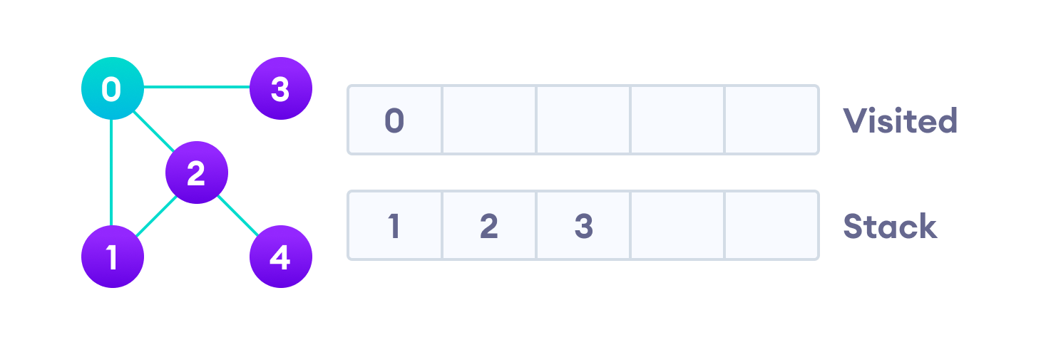
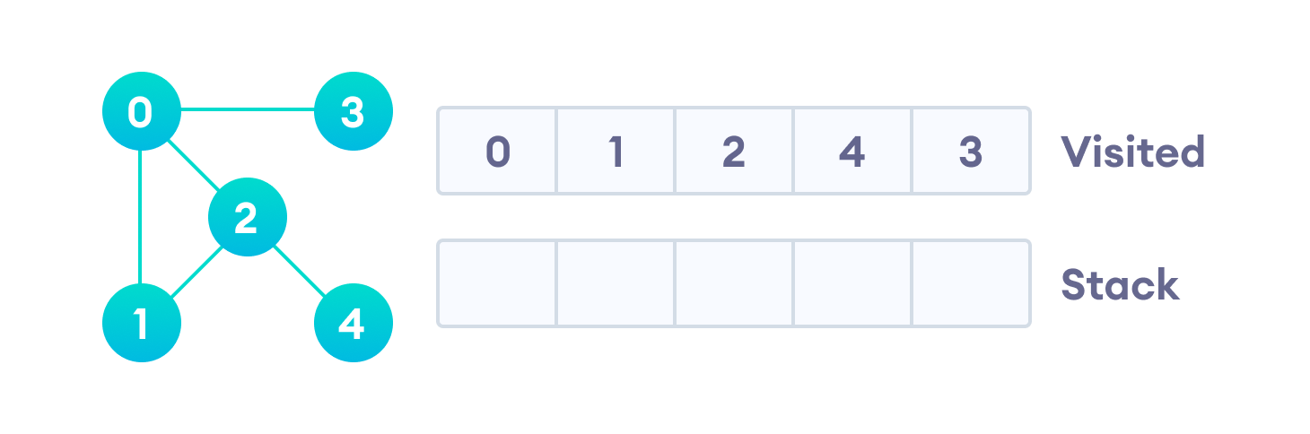
Предлагаю рассмотреть на примере, как работает алгоритм поиска в глубину. Мы будем использовать неориентированный граф с пятью вершинами.

Начнем мы с вершины “0”. В первую очередь алгоритм поиска в глубину поместит ее саму в список “Пройденные” (на изображении “Visited”), а ее смежные вершины — в стек.

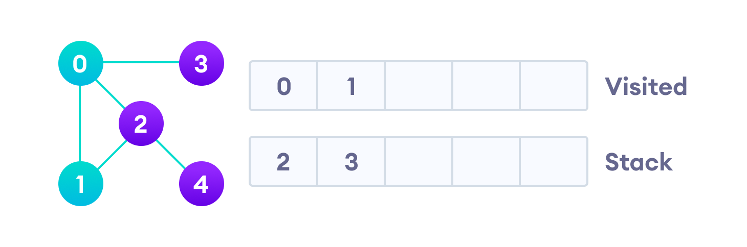
Затем мы берем следующий элемент сверху стека, т.е. к вершину “1”, и переходим к ее соседним вершинам. Поскольку вершина “0” уже пройдена, следующая вершина “2”.

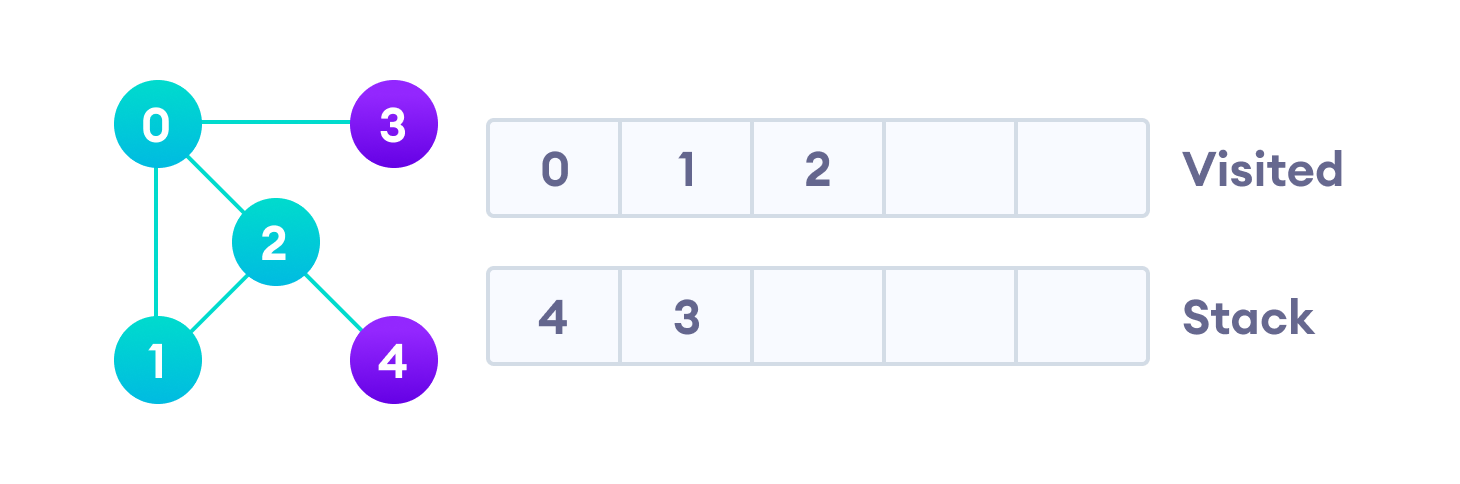
Вершина “2” смежна непройденной вершине “4”, следовательно мы добавляем ее наверх стека и проходим ее.

После того, как мы пройдем последний элемент (вершину “3”), в стеке не останется непройденных смежных вершин, и таким образом мы завершили обход графа в глубину.

Псевдокод поиска в глубину (рекурсивная реализация)

Ниже представлен псевдокод для алгоритма поиска в глубину. Обратите внимание, что в функции init() необходимо запускать функцию DFS на каждой вершине. Это связано с тем, что граф может иметь две разные несвязанные части, поэтому для того, чтобы убедиться, что мы покрываем каждую вершину, мы должны запускать алгоритм поиска в глубину на каждой вершине.

DFS(G, u) u.visited = true for each v ∈ G.Adj[u] if v.visited == false DFS(G,v) init()

Реализация поиска в глубину на Python, Java и C/C++

Ниже приведены примеры реально кода алгоритма поиска в глубину. Код был упрощен, чтобы мы могли сфокусироваться на самом алгоритме, а не на других деталях.

# Алгоритм поиска в глубину на Python # Алгоритм def dfs(graph, start, visited=None): if visited is None: visited = set() visited.add(start) print(start) for next in graph[start] - visited: dfs(graph, next, visited) return visited graph = dfs(graph, '0')

// Алгоритм поиска в глубину на Java import java.util.*; class Graph < private LinkedListadjLists[]; private boolean visited[]; // Создание графа Graph(int vertices) < adjLists = new LinkedList[vertices]; visited = new boolean[vertices]; for (int i = 0; i < vertices; i++) adjLists[i] = new LinkedList(); > // Добавление ребер void addEdge(int src, int dest) < adjLists[src].add(dest); >// Алгоритм void DFS(int vertex) < visited[vertex] = true; System.out.print(vertex + " "); Iteratorite = adjLists[vertex].listIterator(); while (ite.hasNext()) < int adj = ite.next(); if (!visited[adj]) DFS(adj); >> public static void main(String args[]) < Graph g = new Graph(4); g.addEdge(0, 1); g.addEdge(0, 2); g.addEdge(1, 2); g.addEdge(2, 3); System.out.println("Following is Depth First Traversal"); g.DFS(2); >> 

// Алгоритм поиска в глубину на C #include #include struct node < int vertex; struct node* next; >; struct node* createNode(int v); struct Graph < int numVertices; int* visited; // Нам нужен int** для хранения двумерного массива. // Аналогично, нам нужна структура node** для хранения массива связанных списков. struct node** adjLists; >; // Алгоритм void DFS(struct Graph* graph, int vertex) < struct node* adjList = graph->adjLists[vertex]; struct node* temp = adjList; graph->visited[vertex] = 1; printf("Visited %d \n", vertex); while (temp != NULL) < int connectedVertex = temp->vertex; if (graph->visited[connectedVertex] == 0) < DFS(graph, connectedVertex); >temp = temp->next; > > // Создание вершины struct node* createNode(int v) < struct node* newNode = malloc(sizeof(struct node)); newNode->vertex = v; newNode->next = NULL; return newNode; > // Создание графа struct Graph* createGraph(int vertices) < struct Graph* graph = malloc(sizeof(struct Graph)); graph->numVertices = vertices; graph->adjLists = malloc(vertices * sizeof(struct node*)); graph->visited = malloc(vertices * sizeof(int)); int i; for (i = 0; i < vertices; i++) < graph->adjLists[i] = NULL; graph->visited[i] = 0; > return graph; > // Добавление ребра void addEdge(struct Graph* graph, int src, int dest) < // Проводим ребро от начальной вершины ребра графа к конечной вершине ребра графа struct node* newNode = createNode(dest); newNode->next = graph->adjLists[src]; graph->adjLists[src] = newNode; // Проводим ребро из конечной вершины ребра графа в начальную вершину ребра графа newNode = createNode(src); newNode->next = graph->adjLists[dest]; graph->adjLists[dest] = newNode; > // Выводим граф void printGraph(struct Graph* graph) < int v; for (v = 0; v < graph->numVertices; v++) < struct node* temp = graph->adjLists[v]; printf("\n Adjacency list of vertex %d\n ", v); while (temp) < printf("%d ->", temp->vertex); temp = temp->next; > printf("\n"); > > int main()

// Алгоритм прохода в глубину в C++ #include #include using namespace std; class Graph < int numVertices; list*adjLists; bool *visited; public: Graph(int V); void addEdge(int src, int dest); void DFS(int vertex); >; // Инициализация графа Graph::Graph(int vertices) < numVertices = vertices; adjLists = new list[vertices]; visited = new bool[vertices]; > // Добавление ребер void Graph::addEdge(int src, int dest) < adjLists[src].push_front(dest); >// Алгоритм void Graph::DFS(int vertex) < visited[vertex] = true; listadjList = adjLists[vertex]; cout << vertex << " "; list::iterator i; for (i = adjList.begin(); i != adjList.end(); ++i) if (!visited[*i]) DFS(*i); > int main()

Сложность алгоритма поиска в глубину

Временная сложность алгоритма поиска в глубину представлена ​​в виде O(V + E), где V — количество вершин, а E — количество ребер.

Пространственная сложность алгоритма равна O(V).

Применения алгоритма

1. Для поиска пути.
2. Для проверки двудольности графа.
3. Для поиска сильно связанных компонентов графа.
4. Для обнаружения циклов в графе.

Приглашаем всех желающих на открытый урок в OTUS «Теория графов. Термины и определения. Основные алгоритмы», регистрация доступна по ссылке.

Источник