Moving average model python

Time Series analysis tsa ¶

statsmodels.tsa contains model classes and functions that are useful for time series analysis. Basic models include univariate autoregressive models (AR), vector autoregressive models (VAR) and univariate autoregressive moving average models (ARMA). Non-linear models include Markov switching dynamic regression and autoregression. It also includes descriptive statistics for time series, for example autocorrelation, partial autocorrelation function and periodogram, as well as the corresponding theoretical properties of ARMA or related processes. It also includes methods to work with autoregressive and moving average lag-polynomials. Additionally, related statistical tests and some useful helper functions are available.

Estimation is either done by exact or conditional Maximum Likelihood or conditional least-squares, either using Kalman Filter or direct filters.

Currently, functions and classes have to be imported from the corresponding module, but the main classes will be made available in the statsmodels.tsa namespace. The module structure is within statsmodels.tsa is

• stattools : empirical properties and tests, acf, pacf, granger-causality, adf unit root test, kpss test, bds test, ljung-box test and others.
• ar_model : univariate autoregressive process, estimation with conditional and exact maximum likelihood and conditional least-squares
• arima.model : univariate ARIMA process, estimation with alternative methods
• statespace : Comprehensive statespace model specification and estimation. See the statespace documentation .
• vector_ar, var : vector autoregressive process (VAR) and vector error correction models, estimation, impulse response analysis, forecast error variance decompositions, and data visualization tools. See the vector_ar documentation .
• arma_process : properties of arma processes with given parameters, this includes tools to convert between ARMA, MA and AR representation as well as acf, pacf, spectral density, impulse response function and similar
• sandbox.tsa.fftarma : similar to arma_process but working in frequency domain
• tsatools : additional helper functions, to create arrays of lagged variables, construct regressors for trend, detrend and similar.
• filters : helper function for filtering time series
• regime_switching : Markov switching dynamic regression and autoregression models

Some additional functions that are also useful for time series analysis are in other parts of statsmodels, for example additional statistical tests.

Some related functions are also available in matplotlib, nitime, and scikits.talkbox. Those functions are designed more for the use in signal processing where longer time series are available and work more often in the frequency domain.

Descriptive Statistics and Tests¶

Calculate the autocorrelation function.

Источник

Defining the Moving Average Model for Time Series Forecasting in Python

Explore the moving average model and discover how we can use the ACF plot to identify the right MA(q) model for our time series

One of the foundational models for time series forecasting is the moving average model, denoted as MA(q). This is one of the basic statistical models that is a building block of more complex models such as the ARMA, ARIMA, SARIMA and SARIMAX models. A deep understanding of the MA(q) is thus a key step prior to using more complex models to forecast intricate time series.

In this article, we first define the moving average process and explore its inner workings. We then use a dataset to apply our knowledge and use the ACF plot to determine the order of an MA(q) model.

This article is an excerpt of my upcoming book Time Series Forecasting in Python. If you are interested in learning more about time series forecasting, using both statistical and deep learning models with applied scenarios, you can learn more here.

Prerequisites

You can grab the dataset here. Note that the data is synthetic, as we rarely observe real-life time series that can be modeled with a pure moving average process. This dataset is thus for learning purposes.

The full source code is available here.

Defining the moving average process

A moving average process, or the moving average model, states that the current value is linearly dependent on the current and past error terms. Again, the error terms are assumed to be mutually independent and normally distributed, just like white noise.

A moving average model is denoted as MA(q) where q is the order. The model expresses the present value as a linear combination of the mean of the series (mu), the present error term (epsilon), and past error terms (epsilon). The magnitude of the impact of past errors on the present value is quantified using a coefficient denoted with theta…

Источник

MA Model in Python

The moving average model, or MA model, predicts a value at a particular time using previous errors. The model relies on the average of previous time serries and correlations between errors that suggest we can predict the current value based on previous errors. In this article, we will learn how to build an Moving Average model in Python.

The Model Math

Let’s take a brief look at the mathematical definition. We predicted value of an MA model follow this equation for MA(1)

• μ \mu μ is the average of previous values
• θ 1 \theta_1 θ 1 ​ is our coefficient for Moving Average
• e t − 1 e_ e t − 1 ​ is the previous error at time t-1
• e t e_t e t ​ is the error of the current time

If we want to expand to MA(2) and more, we get add another lag, previous time value, and another coefficient. For example.

y t = μ + θ 1 ∗ e t − 1 + θ 2 ∗ e t − 2 + e t y_t = \mu + \theta_1 * e_ + \theta_2 * e_ + e_t y t ​ = μ + θ 1 ​ ∗ e t − 1 ​ + θ 2 ​ ∗ e t − 2 ​ + e t ​

Let’s say we have an MA model and we have the following sales for two months: [ 200 , 200, 200 , 300] and we have the error values from the previous predicted minus the actual value [20, 30]. We can then predict y_3 for the third month as follows:

y 3 = ( 200 + 300 ) / 2 + θ a ∗ 30 + e t y_3 = (200+300)/2 + \theta_a * 30 + e_t y 3 ​ = ( 200 + 300 ) /2 + θ a ​ ∗ 30 + e t ​

Where we find \mu and theta by performing linear regression on the data set and the e_t is assumed to be sampled from a normal distribution.

Dataset

To test out ARIMA style models, we can use ArmaProcess function. This will simulate a model for us, so that we can test and verify our technique. Let’s start with an MA(1) model using the code below. To create an arr model, we set the model params to have order c(0, 0, 1) . This order represents 0 AR term, 0 diff terms, and 1 MA terms. We also pass the value of the MA parameter which is .9.

from statsmodels.tsa.arima_process import ArmaProcess import numpy as np ar = np.array([1]) ma = np.array([1, -.9]) ma_simulater = ArmaProcess(ar, ma) ma_sim = ar_simulater.generate_sample(nsample=100)

import matplotlib.pyplot as plt plt.plot(ma_sim)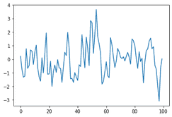

Viewing the ACF or PACF

When trying to model ARMA models, we usually use the ACF or PACF. It is worth noting that before this, you will want to have remove trend and seasonality. We will have a full article on ARIMA modeling later on. For MR models, the ACF will help us determine the component, but we also need to confirm the PACF does not drop off as well.

We start with the ACF plot. We see a drastic drop off after the first lag.

from statsmodels.graphics import tsaplots tsaplots.plot_acf(ma_sim)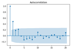

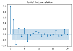
We now look at the PACF plot. We don’t see an immediate drop off and later lags seem to be correlated. This is consistent for an MA model.

from statsmodels.graphics import tsaplots tsaplots.plot_pacf(ma_sim)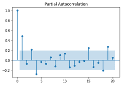

Fitting the Model

We can use the built in arima function to model our data. We pass in our data set and the order we want to model.

## Ignore some warnings import warnings warnings.filterwarnings('ignore')

from statsmodels.tsa.arima_model import ARMA mod = ARMA(ma_sim, order=(0, 1)) res = mod.fit() res.summary()

ARMA Model Results

Dep. Variable:	y	No. Observations:	100
Model:	ARMA(0, 1)	Log Likelihood	-142.178
Method:	css-mle	S.D. of innovations	1.000
Date:	Mon, 09 Aug 2021	AIC	290.355
Time:	07:30:10	BIC	298.171
Sample:	0	HQIC	293.518

coef	std err	z	P>|z|	[0.025	0.975]
const	-0.0273	0.163	-0.168	0.867	-0.347	0.292
ma.L1.y	0.6366	0.093	6.830	0.000	0.454	0.819

Roots

Real	Imaginary	Modulus	Frequency
MA.1	-1.5709	+0.0000j	1.5709	0.5000

We can see the ar1 was modeled at .68 which is very close to the .7 we simulated. Another value to check here is the aic, 147.11, which we would use to confirm the model compared to others.

We can now forecast our model using the plot_predict function. Here we predict 20 time values forward and plot the new values.

res.plot_predict(start=0, end = 120)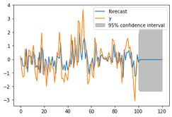

Modeling an MA(2)

Let’s finish with one more example. We will go a bit quick, and use all the steps above.

from statsmodels.tsa.arima_process import ArmaProcess import numpy as np ar2 = np.array([1]) ma2 = np.array([1, -.7, .4]) ma2_simulater = ArmaProcess(ar2, ma2) ma2_sim = ar_simulater.generate_sample(nsample=100)

import matplotlib.pyplot as plt plt.plot(ma2_sim)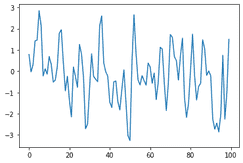

from statsmodels.graphics import tsaplots tsaplots.plot_acf(ma2_sim)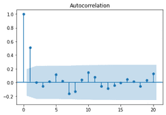

from statsmodels.tsa.arima_model import ARMA mod = ARMA(ma2_sim, order=(2, 0)) res = mod.fit() res.summary()

ARMA Model Results

Dep. Variable:	y	No. Observations:	100
Model:	ARMA(2, 0)	Log Likelihood	-147.638
Method:	css-mle	S.D. of innovations	1.056
Date:	Mon, 09 Aug 2021	AIC	303.276
Time:	07:30:58	BIC	313.697
Sample:	0	HQIC	307.494

coef	std err	z	P>|z|	[0.025	0.975]
const	-0.1790	0.161	-1.113	0.266	-0.494	0.136
ar.L1.y	0.7198	0.094	7.651	0.000	0.535	0.904
ar.L2.y	-0.3770	0.093	-4.033	0.000	-0.560	-0.194

Roots

Real	Imaginary	Modulus	Frequency
AR.1	0.9546	-1.3195j	1.6286	-0.1503
AR.2	0.9546	+1.3195j	1.6286	0.1503

res.plot_predict(start=0, end = 120)

Источник