statsmodels.stats.diagnostic.acorr_ljungbox
The data series. The data is demeaned before the test statistic is computed.
lags , default None
If lags is an integer then this is taken to be the largest lag that is included, the test result is reported for all smaller lag length. If lags is a list or array, then all lags are included up to the largest lag in the list, however only the tests for the lags in the list are reported. If lags is None, then the default maxlag is min(10, nobs // 5). The default number of lags changes if period is set.
boxpierce bool , default False
If true, then additional to the results of the Ljung-Box test also the Box-Pierce test results are returned.
model_df int , default 0
Number of degrees of freedom consumed by the model. In an ARMA model, this value is usually p+q where p is the AR order and q is the MA order. This value is subtracted from the degrees-of-freedom used in the test so that the adjusted dof for the statistics are lags — model_df. If lags — model_df
period int , default None
The period of a Seasonal time series. Used to compute the max lag for seasonal data which uses min(2*period, nobs // 5) if set. If None, then the default rule is used to set the number of lags. When set, must be >= 2.
auto_lag bool , default False
Flag indicating whether to automatically determine the optimal lag length based on threshold of maximum correlation value.
- lb_stat — The Ljung-Box test statistic.
- lb_pvalue — The p-value based on chi-square distribution. The p-value is computed as 1 — chi2.cdf(lb_stat, dof) where dof is lag — model_df. If lag — model_df
- bp_stat — The Box-Pierce test statistic.
- bp_pvalue — The p-value based for Box-Pierce test on chi-square distribution. The p-value is computed as 1 — chi2.cdf(bp_stat, dof) where dof is lag — model_df. If lag — model_df
Results from linear regression models.
Ljung-Box test statistic computed from estimated autocorrelations.
Ljung-Box and Box-Pierce statistic differ in their scaling of the autocorrelation function. Ljung-Box test is has better finite-sample properties.
Green, W. “Econometric Analysis,” 5th ed., Pearson, 2003.
J. Carlos Escanciano, Ignacio N. Lobato “An automatic Portmanteau test for serial correlation”., Volume 151, 2009.
>>> import statsmodels.api as sm >>> data = sm.datasets.sunspots.load_pandas().data >>> res = sm.tsa.ARMA(data["SUNACTIVITY"], (1,1)).fit(disp=-1) >>> sm.stats.acorr_ljungbox(res.resid, lags=[10], return_df=True) lb_stat lb_pvalue 10 214.106992 1.827374e-40 statsmodels.stats.diagnostic.acorr_ljungbox
The data series. The data is demeaned before the test statistic is computed.
lags , default None
If lags is an integer then this is taken to be the largest lag that is included, the test result is reported for all smaller lag length. If lags is a list or array, then all lags are included up to the largest lag in the list, however only the tests for the lags in the list are reported. If lags is None, then the default maxlag is min(10, nobs // 5). The default number of lags changes if period is set.
boxpierce bool , default False
If true, then additional to the results of the Ljung-Box test also the Box-Pierce test results are returned.
model_df int , default 0
Number of degrees of freedom consumed by the model. In an ARMA model, this value is usually p+q where p is the AR order and q is the MA order. This value is subtracted from the degrees-of-freedom used in the test so that the adjusted dof for the statistics are lags — model_df. If lags — model_df
period int , default None
The period of a Seasonal time series. Used to compute the max lag for seasonal data which uses min(2*period, nobs // 5) if set. If None, then the default rule is used to set the number of lags. When set, must be >= 2.
auto_lag bool , default False
Flag indicating whether to automatically determine the optimal lag length based on threshold of maximum correlation value.
- lb_stat — The Ljung-Box test statistic.
- lb_pvalue — The p-value based on chi-square distribution. The p-value is computed as 1 — chi2.cdf(lb_stat, dof) where dof is lag — model_df. If lag — model_df
- bp_stat — The Box-Pierce test statistic.
- bp_pvalue — The p-value based for Box-Pierce test on chi-square distribution. The p-value is computed as 1 — chi2.cdf(bp_stat, dof) where dof is lag — model_df. If lag — model_df
Results from linear regression models.
Ljung-Box test statistic computed from estimated autocorrelations.
Ljung-Box and Box-Pierce statistic differ in their scaling of the autocorrelation function. Ljung-Box test is has better finite-sample properties.
Green, W. “Econometric Analysis,” 5th ed., Pearson, 2003.
J. Carlos Escanciano, Ignacio N. Lobato “An automatic Portmanteau test for serial correlation”., Volume 151, 2009.
>>> import statsmodels.api as sm >>> data = sm.datasets.sunspots.load_pandas().data >>> res = sm.tsa.ARMA(data["SUNACTIVITY"], (1,1)).fit(disp=-1) >>> sm.stats.acorr_ljungbox(res.resid, lags=[10], return_df=True) lb_stat lb_pvalue 10 214.106992 1.827374e-40 Statistic and Statistical Tests
When estimating model parameters using maximum likelihood estimation, it is possible to increase the likelihood by adding parameters, which may result in overfitting. The BIC resolves this problem by introducing a penalty term for the number of parameters in the model. This penalty is larger in the BIC than in the related AIC. [wikibic].
A rough approximation [bisp2006] [calinon2007] of the Bayesian Information Criterion (BIC) is given by
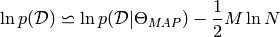


The number of free parameters is given by the model used.

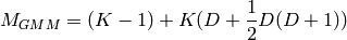
The number of parameters in a Gaussian Mixture Model (GMM) with clusters and a full covariance matrix, can be found by counting the free parameters in the means and covariances, which should give [calinon2007]

| [bisp2006] | Christopher M. Bishop. Pattern Recognition and Machine Learning (Infor- mation Science and Statistics). Springer-Verlag New York, Inc., Secaucus, NJ, USA, 2006. |
| [calinon2007] | (1, 2) Sylvain Calinon, Florent Guenter, and Aude Billard. On learning, repre- senting, and generalizing a task in a humanoid robot. Systems, Man and Cybernetics, Part B, IEEE Transactions on, 37(2):286-298, 2007. http://programming-by-demonstration.org/papers/Calinon-JSMC2007.pdf |
| [wikibic] | Bayesian information criterion. (2011, February 21). In Wikipedia, The Free Encyclopedia. Retrieved 11:57, March 1, 2011, from http://en.wikipedia.org/w/index.php?title=Bayesian_information_criterion&oldid=415136150 |
Akaike Information Criterion
Sample Autocorrelation
Supposed we have a time series given by 
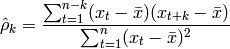


![\hat<\rho></noscript>_k»/> is the sample autocorrelation</p><p>Sample autocorrelation (As used in statistics with normalization)</p><p><strong>x</strong> : 1d numpy array</p><p><strong>k</strong> : int or list of ints</p><blockquote><p>Lags to calculate sample autocorrelation for</p></blockquote><p><strong>res</strong> : scalar or np array</p><blockquote><p>The sample autocorrelation. A scalar value if k is a scalar, and a numpy array if k is a interable.</p></blockquote><h2>Ljung-Box Test¶</h2><p>The Ljung-Box test is a type of statistical test of whether any of a group of autocorrelations of a time series are different from zero. Instead of testing randomness at each distinct lag, it tests the “overall” randomness based on a number of lags [wikiljungbox].</p><p><img decoding=](https://pypr.sourceforge.net/_images/math/72d2567a718898fe6d99e1f0cb202743dc52510b.png)


The Ljung-Box test for determining if the data is independently distributed.
x : 1d numpy array

For significance level , the critical region for rejection of the hypothesis of randomness is [wikiljungbox].

Example
This example uses the sample autocorrelation, acf(. ) , which also is defined in pypr.stattest module.
from pypr.stattest.ljungbox import * import scipy.stats x = np.random.randn(100) #rg = genfromtxt('sunspots/sp.dat') #x = rg[:,1] # Just use number of sun spots, ignore year h = 20 # Number of lags lags = range(h) sa = np.zeros((h)) for k in range(len(lags)): sa[k] = sac(x, k) figure() markerline, stemlines, baseline = stem(lags, sa) grid() title('Sample Autocorrealtion Function (ACF)') ylabel('Sample Autocorrelation') xlabel('Lag') h, pV, Q, cV = lbqtest(x, range(1, 20), alpha=0.1) print 'lag p-value Q c-value rejectH0' for i in range(len(h)): print "%-2d %10.3f %10.3f %10.3f %s" % (i+1, pV[i], Q[i], cV[i], str(h[i]))
The example generates a sample autocorrelation for the sun spot data set, and calculates the Ljung-Box test statistics.

The output should look something similar to this:
lag p-value Q c-value rejectH0 1 0.164 1.935 2.706 False 2 0.378 1.948 4.605 False 3 0.542 2.148 6.251 False 4 0.600 2.752 7.779 False 5 0.718 2.884 9.236 False 6 0.823 2.884 10.645 False 7 0.895 2.885 12.017 False 8 0.941 2.897 13.362 False 9 0.966 2.948 14.684 False 10 0.941 4.132 15.987 False 11 0.888 5.781 17.275 False 12 0.922 5.887 18.549 False 13 0.724 9.625 19.812 False 14 0.744 10.242 21.064 False 15 0.756 10.949 22.307 False 16 0.746 11.969 23.542 False 17 0.801 11.979 24.769 False 18 0.847 12.008 25.989 False 19 0.885 12.020 27.204 False
| [wikiljungbox] | (1, 2, 3) Ljung–Box test. (2011, February 17). In Wikipedia, The Free Encyclopedia. Retrieved 12:46, February 23, 2011, from http://en.wikipedia.org/w/index.php?title=Ljung%E2%80%93Box_test&oldid=414387240 |
| [adres1766] | http://adorio-research.org/wordpress/?p=1766 |
| [mathworks-lbqtest] | http://www.mathworks.com/help/toolbox/econ/lbqtest.html |
Box-Pierce Test
The Ljung–Box test that we have just looked at is a preferred version of the Box–Pierce test, because the Box–Pierce statistic has poor performance in small samples [wikilboxpierce].
