- Least Squares Linear Regression In Python
- Algorithm
- Least Squares Linear Regression With Python Example
- Sample Dataset
- Least Squares Formula
- Least Squares Linear Regression By Hand
- Least Squares Linear Regression With Python Sklearn
- Plot Data And Regression Line In Python
- Partial Least Squares Regression in Python
- Difference between PCR and PLS regression
- PLS Python code
- Ordinary Least Squares (OLS) using statsmodels
Least Squares Linear Regression In Python
As the name implies, the method of Least Squares minimizes the sum of the squares of the residuals between the observed targets in the dataset, and the targets predicted by the linear approximation. In this proceeding article, we’ll see how we can go about finding the best fitting line using linear algebra as opposed to something like gradient descent.
Algorithm
Contrary to what I had initially thought, the scikit-learn implementation of Linear Regression minimizes a cost function of the form:
using the singular value decomposition of X.
If you’re already familiar with Linear Regression, you might see some similarities to the preceding equation and the mean square error (MSE).
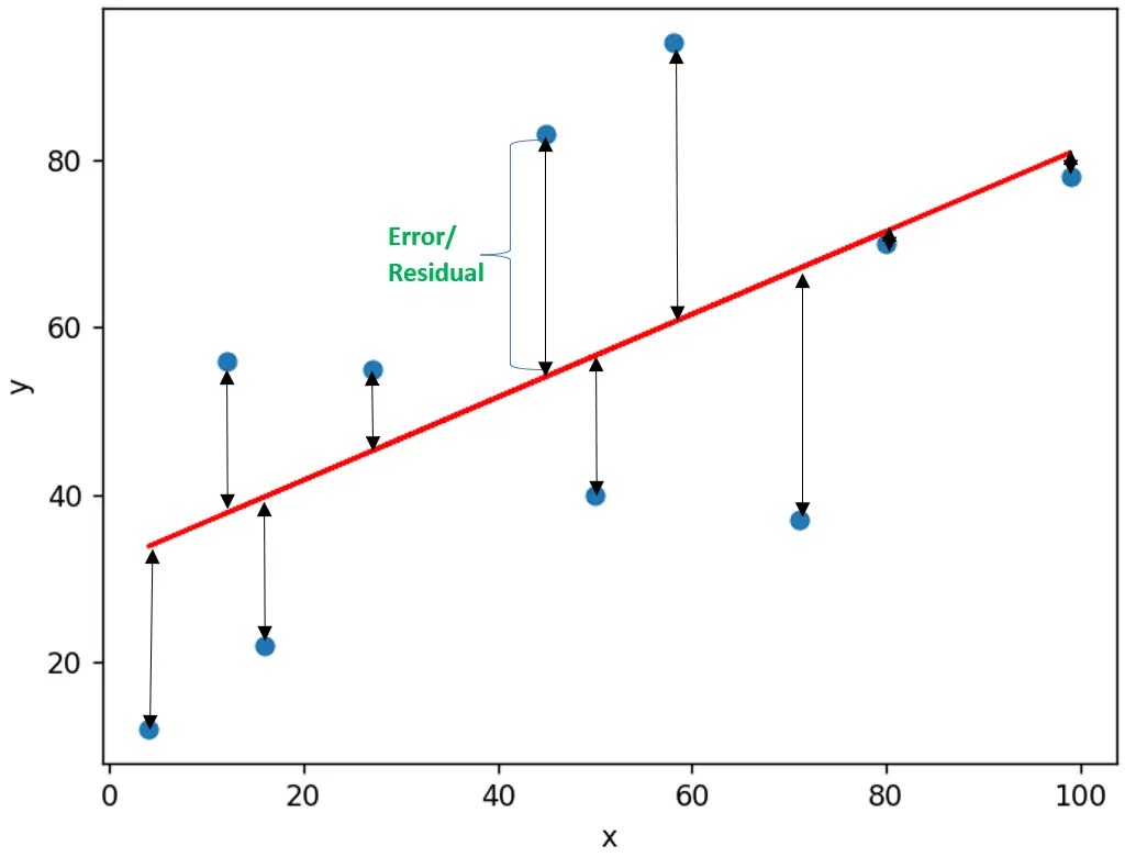
As quick refresher, suppose we had the following scatter plot and regression line.
We calculate the distance from the line to a given data point by subtracting one from the other. We take the square of the difference because we don’t want the predicted values below the actual values to cancel out with those above the actual values. In mathematical terms, the latter can be expressed as follows:
The cost function used in the scikit-learn library is similar, only we’re calculating it simultaneously using matrix operations.
For those of you that have taken a Calculus course, you’ve probably encountered this kind of notation before.
In this case, x is a vector and we are calculating its magnitude.
In the same sense, when we surround the variable for a matrix (i.e. A) by vertical bars, we are saying that we want to go from a matrix of rows and columns to a scalar. There are multiple ways of deriving a scalar from a matrix. Depending on which one is used, you’ll see a different symbol to the right of the variable (the extra 2 in the equation wasn’t put there by accident).
Least Squares Linear Regression With Python Example
This tutorial will show you how to do a least squares linear regression with Python using an example we discussed earlier. Check here to learn what a least squares regression is.
Sample Dataset
We’ll use the following 10 randomly generated data point pairs.
Least Squares Formula
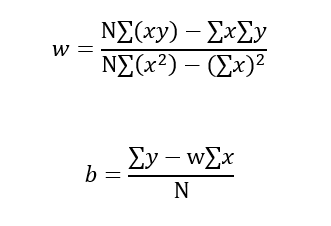
For a least squares problem, our goal is to find a line y = b + wx that best represents/fits the given data points. In other words, we need to find the b and w values that minimize the sum of squared errors for the line.
As a reminder, the following equations will solve the best b (intercept) and w (slope) for us:
Least Squares Linear Regression By Hand
Let’s create two new lists, xy and x_sqrt:
We can then calculate the w (slope) and b (intercept) terms using the above formula:
Least Squares Linear Regression With Python Sklearn
Scikit-learn is a great Python library for data science, and we’ll use it to help us with linear regression. We also need to use numpy library to help with data transformation. Let’s install both using pip, note the library name is sklearn:
In general, sklearn prefers 2D array input over 1D. The x and y lists are considered as 1D, so we have to convert them into 2D arrays using numpy’s reshape() method. Note although the below new x and y still look like 1D arrays after transformation, they are technically 2D because each x and y is now a list of lists.
Our data is in the proper format now, we can create a linear regression and “fit” (another term is “train”) the model. Under the hood, sklearn will perform the w and b calculations.
We can check the intercept (b) and slope(w) values. Note by sklearn‘s naming convention, attributes followed by an underscore “_” implies they are estimated from the data.
As shown above, the values match our previously hand-calculated values.
Plot Data And Regression Line In Python
We’ll use the matplotlib library for plotting, get it with pip if you don’t have it yet:
Matplotlib is probably the most well-known plotting library in Python. It provides great flexibility for customization if you know what you are doing 🙂
Partial Least Squares Regression in Python
Hi everyone, and thanks for stopping by. Today we are going to present a worked example of Partial Least Squares Regression in Python on real world NIR data.
PLS, acronym of Partial Least Squares, is a widespread regression technique used to analyse near-infrared spectroscopy data. If you know a bit about NIR spectroscopy, you sure know very well that NIR is a secondary method and NIR data needs to be calibrated against primary reference data of the parameter one seeks to measure. This calibration must be done the first time only. Once the calibration is done, and is robust, one can go ahead and use NIR data to predict values of the parameter of interest.
In previous posts we discussed qualitative analysis of NIR data by Principal Component Analysis (PCA), and how one can make a step further and build a regression model using Principal Component Regression (PCR). You can check out some of our related posts here.
PCR is quite simply a regression model built using a number of principal components derived using PCA. In our last post on PCR, we discussed how PCR is a nice and simple technique, but limited by the fact that it does not take into account anything other than the regression data. That is, our primary reference data are not considered when building a PCR model. That is obviously not optimal, and PLS is a way to fix that.
In this post I am going to show you how to build a simple regression model using PLS in Python. This is the overview of what we are going to do.
- Mathematical introduction on the difference between PCR and PLS regression (for the bravest)
- Present the basic code for PLS
- Discuss the data we want to analyse and the pre-processing required. We are going to use NIR spectra of fresh peach fruits having an associated value of Brix (same as for the PCR post). That is the quantity we want to calibrate for.
- We will build our model using a cross-validation approach
Difference between PCR and PLS regression
Before working on some code, let’s very briefly discuss the mathematical difference between PCR and PLS. I decided to include this description because it may be of interest for some of our readers, however this is not required to understand the code. Feel free to skip this section altogether if you’re not feeling like dealing with math right now. I won’t hold it against you.
Both PLS and PCR perform multiple linear regression, that is they build a linear model, Y=XB+E . Using a common language in statistics, X is the predictor and Y is the response. In NIR analysis, X is the set of spectra, Y is the quantity – or quantities- we want to calibrate for (in our case the brix values). Finally E is an error.
As we discussed in the PCR post, the matrix X contains highly correlated data and this correlation (unrelated to brix) may obscure the variations we want to measure, that is the variations of the brix content. Both PCR and PLS will get rid of the correlation.
In PCR (if you’re tuning in now, that is Principal Component Regression) the set of measurements X is transformed into an equivalent set X’=XW by a linear transformation W , such that all the new ‘spectra’ (which are the principal components) are linearly independent. In statistics X’ is called the factor scores. The linear transformation in PCR is such that it minimises the covariance between the different rows of X’ . That means this process only uses the spectral data, not the response values.
This is the key difference between PCR and PLS regression. PLS is based on finding a similar linear transformation, but accomplishes the same task by maximising the covariance between Y and X’ . In other words, PLS takes into account both spectra and response values and in doing so will improve on some of the limitations on PCR. For these reasons PLS is one of the staples of modern chemometrics.
I’m not sure if that makes any sense to you, but that was my best shot at explaining the difference without writing down too many equations.
PLS Python code
OK, here’s the basic code to run PLS in cross-validation, based on Python 3.5.2.
Ordinary Least Squares (OLS) using statsmodels
In this article, we will use Python’s statsmodels module to implement Ordinary Least Squares(OLS) method of linear regression.
Introduction :
A linear regression model establishes the relation between a dependent variable(y) and at least one independent variable(x) as : 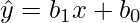
 such that, the total sum of squares of the difference between the calculated and observed values of y, is minimised.
Formula for OLS:
Where,
 = predicted value for the ith observation
  = actual value for the ith observation
  = error/residual for the ith observation
n = total number of observations
To get the values of and  which minimise S, we can take a partial derivative for each coefficient and equate it to zero.
Modules used :
- statsmodels : provides classes and functions for the estimation of many different statistical models.
- Matplotlib : a comprehensive library used for creating static and interactive graphs and visualisations.
- First we define the variables x and y. In the example below, the variables are read from a csv file using pandas. The file used in the example can be downloaded here.
- Next, We need to add the constant to the equation using the add_constant() method.
- The OLS() function of the statsmodels.api module is used to perform OLS regression. It returns an OLS object. Then fit() method is called on this object for fitting the regression line to the data.
- The summary() method is used to obtain a table which gives an extensive description about the regression results
Syntax : statsmodels.api.OLS(y, x)
Parameters :
- y : the variable which is dependent on x
- x : the independent variable