numpy.random.laplace#
Draw samples from the Laplace or double exponential distribution with specified location (or mean) and scale (decay).
The Laplace distribution is similar to the Gaussian/normal distribution, but is sharper at the peak and has fatter tails. It represents the difference between two independent, identically distributed exponential random variables.
New code should use the laplace method of a Generator instance instead; please see the Quick Start .
The position, \(\mu\) , of the distribution peak. Default is 0.
scale float or array_like of floats, optional
\(\lambda\) , the exponential decay. Default is 1. Must be non- negative.
size int or tuple of ints, optional
Output shape. If the given shape is, e.g., (m, n, k) , then m * n * k samples are drawn. If size is None (default), a single value is returned if loc and scale are both scalars. Otherwise, np.broadcast(loc, scale).size samples are drawn.
Returns : out ndarray or scalar
Drawn samples from the parameterized Laplace distribution.
which should be used for new code.
It has the probability density function
The first law of Laplace, from 1774, states that the frequency of an error can be expressed as an exponential function of the absolute magnitude of the error, which leads to the Laplace distribution. For many problems in economics and health sciences, this distribution seems to model the data better than the standard Gaussian distribution.
Abramowitz, M. and Stegun, I. A. (Eds.). “Handbook of Mathematical Functions with Formulas, Graphs, and Mathematical Tables, 9th printing,” New York: Dover, 1972.
Kotz, Samuel, et. al. “The Laplace Distribution and Generalizations, “ Birkhauser, 2001.
Weisstein, Eric W. “Laplace Distribution.” From MathWorld–A Wolfram Web Resource. http://mathworld.wolfram.com/LaplaceDistribution.html
Draw samples from the distribution
>>> loc, scale = 0., 1. >>> s = np.random.laplace(loc, scale, 1000)
Display the histogram of the samples, along with the probability density function:
>>> import matplotlib.pyplot as plt >>> count, bins, ignored = plt.hist(s, 30, density=True) >>> x = np.arange(-8., 8., .01) >>> pdf = np.exp(-abs(x-loc)/scale)/(2.*scale) >>> plt.plot(x, pdf)
Plot Gaussian for comparison:
>>> g = (1/(scale * np.sqrt(2 * np.pi)) * . np.exp(-(x - loc)**2 / (2 * scale**2))) >>> plt.plot(x,g)
scipy.ndimage.laplace#
N-D Laplace filter based on approximate second derivatives.
Parameters : input array_like
output array or dtype, optional
The array in which to place the output, or the dtype of the returned array. By default an array of the same dtype as input will be created.
mode str or sequence, optional
The mode parameter determines how the input array is extended when the filter overlaps a border. By passing a sequence of modes with length equal to the number of dimensions of the input array, different modes can be specified along each axis. Default value is ‘reflect’. The valid values and their behavior is as follows:
‘reflect’ (d c b a | a b c d | d c b a)
The input is extended by reflecting about the edge of the last pixel. This mode is also sometimes referred to as half-sample symmetric.
‘constant’ (k k k k | a b c d | k k k k)
The input is extended by filling all values beyond the edge with the same constant value, defined by the cval parameter.
‘nearest’ (a a a a | a b c d | d d d d)
The input is extended by replicating the last pixel.
‘mirror’ (d c b | a b c d | c b a)
The input is extended by reflecting about the center of the last pixel. This mode is also sometimes referred to as whole-sample symmetric.
‘wrap’ (a b c d | a b c d | a b c d)
The input is extended by wrapping around to the opposite edge.
For consistency with the interpolation functions, the following mode names can also be used:
This is a synonym for ‘constant’.
This is a synonym for ‘reflect’.
This is a synonym for ‘wrap’.
cval scalar, optional
Value to fill past edges of input if mode is ‘constant’. Default is 0.0.
>>> from scipy import ndimage, datasets >>> import matplotlib.pyplot as plt >>> fig = plt.figure() >>> plt.gray() # show the filtered result in grayscale >>> ax1 = fig.add_subplot(121) # left side >>> ax2 = fig.add_subplot(122) # right side >>> ascent = datasets.ascent() >>> result = ndimage.laplace(ascent) >>> ax1.imshow(ascent) >>> ax2.imshow(result) >>> plt.show()
scipy.stats.laplace
Continuous random variables are defined from a standard form and may require some shape parameters to complete its specification. Any optional keyword parameters can be passed to the methods of the RV object as given below:
x : array_like
q : array_like
lower or upper tail probability
loc : array_like, optional
location parameter (default=0)
scale : array_like, optional
size : int or tuple of ints, optional
shape of random variates (default computed from input arguments )
moments : str, optional
composed of letters [‘mvsk’] specifying which moments to compute where ‘m’ = mean, ‘v’ = variance, ‘s’ = (Fisher’s) skew and ‘k’ = (Fisher’s) kurtosis. (default=’mv’)
Alternatively, the object may be called (as a function) to fix the shape,
location, and scale parameters returning a “frozen” continuous RV object:
rv = laplace(loc=0, scale=1)
The probability density function for laplace is:
>>> from scipy.stats import laplace >>> import matplotlib.pyplot as plt >>> fig, ax = plt.subplots(1, 1)
Calculate a few first moments:
>>> mean, var, skew, kurt = laplace.stats(moments='mvsk')
Display the probability density function ( pdf ):
>>> x = np.linspace(laplace.ppf(0.01), . laplace.ppf(0.99), 100) >>> ax.plot(x, laplace.pdf(x), . 'r-', lw=5, alpha=0.6, label='laplace pdf')
Alternatively, freeze the distribution and display the frozen pdf:
>>> rv = laplace() >>> ax.plot(x, rv.pdf(x), 'k-', lw=2, label='frozen pdf')
Check accuracy of cdf and ppf :
>>> vals = laplace.ppf([0.001, 0.5, 0.999]) >>> np.allclose([0.001, 0.5, 0.999], laplace.cdf(vals)) True
And compare the histogram:
>>> ax.hist(r, normed=True, histtype='stepfilled', alpha=0.2) >>> ax.legend(loc='best', frameon=False) >>> plt.show()
| rvs(loc=0, scale=1, size=1) | Random variates. |
| pdf(x, loc=0, scale=1) | Probability density function. |
| logpdf(x, loc=0, scale=1) | Log of the probability density function. |
| cdf(x, loc=0, scale=1) | Cumulative density function. |
| logcdf(x, loc=0, scale=1) | Log of the cumulative density function. |
| sf(x, loc=0, scale=1) | Survival function (1-cdf — sometimes more accurate). |
| logsf(x, loc=0, scale=1) | Log of the survival function. |
| ppf(q, loc=0, scale=1) | Percent point function (inverse of cdf — percentiles). |
| isf(q, loc=0, scale=1) | Inverse survival function (inverse of sf). |
| moment(n, loc=0, scale=1) | Non-central moment of order n |
| stats(loc=0, scale=1, moments=’mv’) | Mean(‘m’), variance(‘v’), skew(‘s’), and/or kurtosis(‘k’). |
| entropy(loc=0, scale=1) | (Differential) entropy of the RV. |
| fit(data, loc=0, scale=1) | Parameter estimates for generic data. |
| expect(func, loc=0, scale=1, lb=None, ub=None, conditional=False, ** kwds) | Expected value of a function (of one argument) with respect to the distribution. |
| median(loc=0, scale=1) | Median of the distribution. |
| mean(loc=0, scale=1) | Mean of the distribution. |
| var(loc=0, scale=1) | Variance of the distribution. |
| std(loc=0, scale=1) | Standard deviation of the distribution. |
| interval(alpha, loc=0, scale=1) | Endpoints of the range that contains alpha percent of the distribution |
Scipy stats package
A variety of functionality for dealing with random numbers can be found in the scipy.stats package.
from scipy import stats import matplotlib.pyplot as plt import numpy as np
Distributions
There are over 100 continuous (univariate) distributions and about 15 discrete distributions provided by scipy
To avoid confusion with a norm in linear algebra we’ll import stats.norm as normal
from scipy.stats import norm as normal
A normal distribution with mean \(\mu\) and variance \(\sigma^2\) has a probability density function \begin \frac> e^ <-(x-\mu)^2 / 2\sigma^2>\end
# bounds of the distribution accessed using fields a and b normal.a, normal.b
# mean and variance normal.mean(), normal.var()
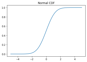
# Cumulative distribution function (CDF) x = np.linspace(-5,5,100) y = normal.cdf(x) plt.plot(x, y) plt.title('Normal CDF');
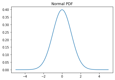
# Probability density function (PDF) x = np.linspace(-5,5,100) y = normal.pdf(x) plt.plot(x, y) plt.title('Normal PDF');
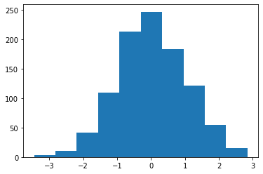
You can sample from a distribution using the rvs method (random variates)
X = normal.rvs(size=1000) plt.hist(X);
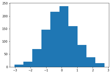
You can set a global random state using np.random.seed or by passing in a random_state argument to rvs
X = normal.rvs(size=1000, random_state=0) plt.hist(X);
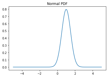
To shift and scale any distribution, you can use the loc and scale keyword arguments
X = normal.rvs(size=1000, random_state=0, loc=1.0, scale=0.5) plt.hist(X);
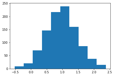
# Probability density function (PDF) x = np.linspace(-5,5,100) y = normal.pdf(x, loc=1.0, scale=0.5) plt.plot(x, y) plt.title('Normal PDF');
You can also “freeze” a distribution so you don’t need to keep passing in the parameters
dist = normal(loc=1.0, scale=0.5) X = dist.rvs(size=1000, random_state=0) plt.hist(X);

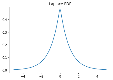
Example: The Laplace Distribution
We’ll review some of the methods we saw above on the Laplace distribution, which has a PDF \begin \frace^ <-|x|>\end
from scipy.stats import laplace
x = np.linspace(-5,5,100) y = laplace.pdf(x) plt.plot(x, y) plt.title('Laplace PDF');
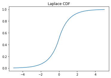
x = np.linspace(-5,5,100) y = laplace.cdf(x) plt.plot(x, y) plt.title('Laplace CDF');
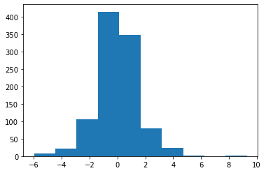
X = laplace.rvs(size=1000) plt.hist(X);
Discrete Distributions
Discrete distributions have many of the same methods as continuous distributions. One notable difference is that they have a probability mass function (PMF) instead of a PDF.
We’ll look at the Poisson distribution as an example
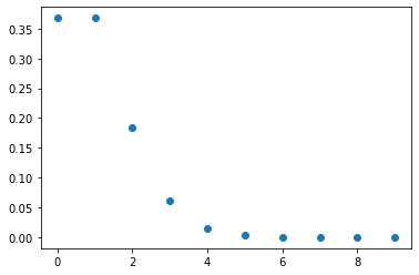
from scipy.stats import poisson dist = poisson(1) # parameter 1
x = np.arange(10) y = dist.pmf(x) plt.scatter(x, y);
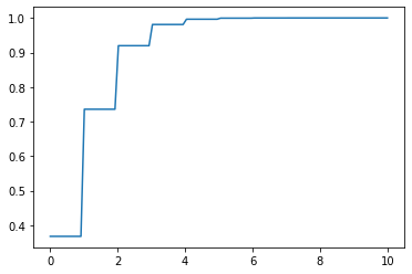
x = np.linspace(0,10, 100) y = dist.cdf(x) plt.plot(x, y);
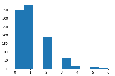
X = dist.rvs(size=1000) plt.hist(X);
Fitting Parameters
You can fit distributions using maximum likelihood estimates
X = normal.rvs(size=100, random_state=0)
(0.059808015534485, 1.0078822447165796)
Statistical Tests
You can also perform a variety of tests. A list of tests available in scipy available can be found here.
the t-test tests whether the mean of a sample differs significantly from the expected mean
Ttest_1sampResult(statistic=0.5904283402851698, pvalue=0.5562489158694675)
The p-value is 0.56, so we would expect to see a sample that deviates from the expected mean at least this much in about 56% of experiments. If we’re doing a hypothesis test, we wouldn’t consider this significant unless the p-value were much smaller (e.g. 0.05)
If we want to test whether two samples could have come from the same distribution, we can use a Kolmogorov-Smirnov (KS) 2-sample test
X0 = normal.rvs(size=1000, random_state=0, loc=5) X1 = normal.rvs(size=1000, random_state=2, loc=5) stats.ks_2samp(X0, X1)
KstestResult(statistic=0.023, pvalue=0.9542189106778983)
We see that the two samples are very likely to come from the same distribution
X0 = normal.rvs(size=1000, random_state=0) X1 = laplace.rvs(size=1000, random_state=2) stats.ks_2samp(X0, X1)
KstestResult(statistic=0.056, pvalue=0.08689937254547132)
When we draw from a different distribution, the p-value is much smaller, indicating that the samples are less likely to have been drawn from the same distribution.
Kernel Density Estimation
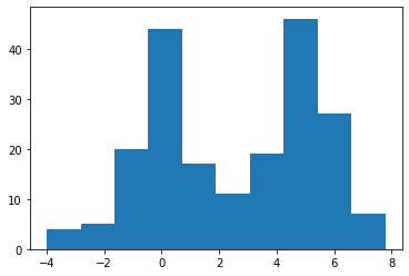
We might also want to estimate a continuous PDF from samples, which can be accomplished using a Gaussian kernel density estimator (KDE)
X = np.hstack((laplace.rvs(size=100), normal.rvs(size=100, loc=5))) plt.hist(X);
A KDE works by creating a function that is the sum of Gaussians centered at each data point. In Scipy this is implemented as an object which can be called like a function
kde = stats.gaussian_kde(X) x = np.linspace(-5,10,500) y = kde(x) plt.plot(x, y) plt.title("KDE");
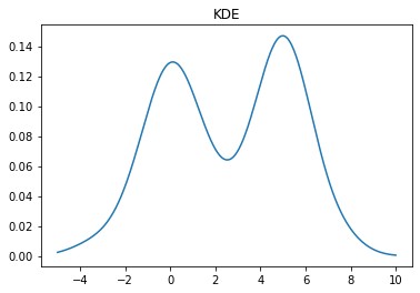
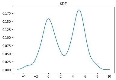
We can change the bandwidth of the Gaussians used in the KDE using the bw_method parameter. You can also pass a function that will set this algorithmically. In the above plot, we see that the peak on the left is a bit smoother than we would expect for the Laplace distribution. We can decrease the bandwidth parameter to make it look sharper:
kde = stats.gaussian_kde(X, bw_method=0.2) x = np.linspace(-5,10,500) y = kde(x) plt.plot(x, y) plt.title("KDE");
If we set the bandwidth too small, then the KDE will look a bit rough.
kde = stats.gaussian_kde(X, bw_method=0.1) x = np.linspace(-5,10,500) y = kde(x) plt.plot(x, y) plt.title("KDE");