scipy.stats.wald#
As an instance of the rv_continuous class, wald object inherits from it a collection of generic methods (see below for the full list), and completes them with details specific for this particular distribution.
The probability density function for wald is:
wald is a special case of invgauss with mu=1 .
The probability density above is defined in the “standardized” form. To shift and/or scale the distribution use the loc and scale parameters. Specifically, wald.pdf(x, loc, scale) is identically equivalent to wald.pdf(y) / scale with y = (x — loc) / scale . Note that shifting the location of a distribution does not make it a “noncentral” distribution; noncentral generalizations of some distributions are available in separate classes.
>>> import numpy as np >>> from scipy.stats import wald >>> import matplotlib.pyplot as plt >>> fig, ax = plt.subplots(1, 1)
Calculate the first four moments:
>>> mean, var, skew, kurt = wald.stats(moments='mvsk')
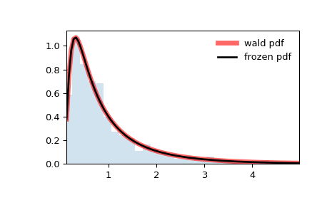
Display the probability density function ( pdf ):
>>> x = np.linspace(wald.ppf(0.01), . wald.ppf(0.99), 100) >>> ax.plot(x, wald.pdf(x), . 'r-', lw=5, alpha=0.6, label='wald pdf')
Alternatively, the distribution object can be called (as a function) to fix the shape, location and scale parameters. This returns a “frozen” RV object holding the given parameters fixed.
Freeze the distribution and display the frozen pdf :
>>> rv = wald() >>> ax.plot(x, rv.pdf(x), 'k-', lw=2, label='frozen pdf')
Check accuracy of cdf and ppf :
>>> vals = wald.ppf([0.001, 0.5, 0.999]) >>> np.allclose([0.001, 0.5, 0.999], wald.cdf(vals)) True
And compare the histogram:
>>> ax.hist(r, density=True, bins='auto', histtype='stepfilled', alpha=0.2) >>> ax.set_xlim([x[0], x[-1]]) >>> ax.legend(loc='best', frameon=False) >>> plt.show()
rvs(loc=0, scale=1, size=1, random_state=None)
pdf(x, loc=0, scale=1)
Probability density function.
logpdf(x, loc=0, scale=1)
Log of the probability density function.
cdf(x, loc=0, scale=1)
Cumulative distribution function.
logcdf(x, loc=0, scale=1)
Log of the cumulative distribution function.
sf(x, loc=0, scale=1)
Survival function (also defined as 1 — cdf , but sf is sometimes more accurate).
logsf(x, loc=0, scale=1)
Log of the survival function.
ppf(q, loc=0, scale=1)
Percent point function (inverse of cdf — percentiles).
isf(q, loc=0, scale=1)
Inverse survival function (inverse of sf ).
moment(order, loc=0, scale=1)
Non-central moment of the specified order.
stats(loc=0, scale=1, moments=’mv’)
Mean(‘m’), variance(‘v’), skew(‘s’), and/or kurtosis(‘k’).
entropy(loc=0, scale=1)
(Differential) entropy of the RV.
Parameter estimates for generic data. See scipy.stats.rv_continuous.fit for detailed documentation of the keyword arguments.
expect(func, args=(), loc=0, scale=1, lb=None, ub=None, conditional=False, **kwds)
Expected value of a function (of one argument) with respect to the distribution.
median(loc=0, scale=1)
Median of the distribution.
mean(loc=0, scale=1)
var(loc=0, scale=1)
Variance of the distribution.
std(loc=0, scale=1)
Standard deviation of the distribution.
interval(confidence, loc=0, scale=1)
Confidence interval with equal areas around the median.
How can I do test wald in Python?
I want to test a hypothesis that «intercept = 0, beta = 1» so I should do wald test and used module ‘statsmodel.formula.api’. But I’m not sure which code is correct when doing wald test.
from statsmodels.datasets import longley import statsmodels.formula.api as smf data = longley.load_pandas().data hypothesis_0 = '(Intercept = 0, GNP = 0)' hypothesis_1 = '(GNP = 0)' hypothesis_2 = '(GNP = 1)' hypothesis_3 = '(Intercept = 0, GNP = 1)' results = smf.ols('TOTEMP ~ GNP', data).fit() wald_0 = results.wald_test(hypothesis_0) wald_1 = results.wald_test(hypothesis_1) wald_2 = results.wald_test(hypothesis_2) wald_3 = results.wald_test(hypothesis_3) print(wald_0) print(wald_1) print(wald_2) print(wald_3) results.summary() I thought hypothesis_3 is right at first. But the result of hypothesis_1 is same with F-test of regression, which represent that the hypothesis ‘intercept = 0 and beta = 0′. So, I thought that the module,’wald_test’ set ‘intercept = 0’ by default. I’m not sure which one is correct. Could you please give me an answer which one is right?
F-test of regression is that all slope coefficients are zero, but leaves the intercept unrestricted, i.e. same as hypothesis_1 in this case.
1 Answer 1
Hypothesis 3 is the correct joint null hypothesis for the wald test. Hypothesis 1 is the same as the F-test in the summary output which is the hypothesis that all slope coefficients are zero.
I changed the example to use artificial data, so we can see the effect of different «true» beta coefficients.
import numpy as np import pandas as pd nobs = 100 np.random.seed(987125) yx = np.random.randn(nobs, 2) beta0 = 0 beta1 = 1 yx[:, 0] += beta0 + beta1 * yx[:, 1] data = pd.DataFrame(yx, columns=['TOTEMP', 'GNP']) hypothesis_0 = '(Intercept = 0, GNP = 0)' hypothesis_1 = '(GNP = 0)' hypothesis_2 = '(GNP = 1)' hypothesis_3 = '(Intercept = 0, GNP = 1)' results = smf.ols('TOTEMP ~ GNP', data).fit() wald_0 = results.wald_test(hypothesis_0) wald_1 = results.wald_test(hypothesis_1) wald_2 = results.wald_test(hypothesis_2) wald_3 = results.wald_test(hypothesis_3) print('H0:', hypothesis_0) print(wald_0) print() print('H0:', hypothesis_1) print(wald_1) print() print('H0:', hypothesis_2) print(wald_2) print() print('H0:', hypothesis_3) print(wald_3) In this case with beta0=0 and beta1=1, both hypothesis 2 and 3 hold. Hypothesis 0 and 1 are not consistent with the simulated data.
The wald test results reject the false and do not reject the true hypotheses, given sample size and effect size should result in high power.
H0: (Intercept = 0, GNP = 0) H0: (GNP = 0) H0: (GNP = 1) H0: (Intercept = 0, GNP = 1)
Similar results can be checked by changing beta0 and beta1.
kwcooper / Wald-Wolfowitz_Runs_Test.py
This file contains bidirectional Unicode text that may be interpreted or compiled differently than what appears below. To review, open the file in an editor that reveals hidden Unicode characters. Learn more about bidirectional Unicode characters
| # Wald-Wolfowitz Runs Test (Actual) |
| # *** For educational purposes only, |
| # use more robust code for actual analysis |
| import math |
| import scipy . stats as st # for pvalue |
| # Example data (Current script only works for binary ints) |
| L = [ 1 , 1 , 1 , 0 , 1 , 1 , 1 , 0 , 0 , 1 , 1 , 0 , 0 , 1 , 1 , 1 , 0 , 1 , 1 , 0 , 0 , 0 , 1 , 0 , 1 , 0 , 0 , 1 , 0 , 0 , 1 , 1 , 1 , 0 , 0 , 0 , 1 ] |
| # Finds runs in data: counts and creates a list of them |
| # TODO: There has to be a more pythonic way to do this. |
| def getRuns ( l ): |
| runsList = [] |
| tmpList = [] |
| for i in l : |
| if len ( tmpList ) == 0 : |
| tmpList . append ( i ) |
| elif i == tmpList [ len ( tmpList ) — 1 ]: |
| tmpList . append ( i ) |
| elif i != tmpList [ len ( tmpList ) — 1 ]: |
| runsList . append ( tmpList ) |
| tmpList = [ i ] |
| runsList . append ( tmpList ) |
| return len ( runsList ), runsList |
| # define the WW runs test described above |
| def WW_runs_test ( R , n1 , n2 , n ): |
| # compute the standard error of R if the null (random) is true |
| seR = math . sqrt ( (( 2 * n1 * n2 ) * ( 2 * n1 * n2 — n )) / (( n ** 2 ) * ( n — 1 )) ) |
| # compute the expected value of R if the null is true |
| muR = (( 2 * n1 * n2 ) / n ) + 1 |
| # test statistic: R vs muR |
| z = ( R — muR ) / seR |
| return z |
| # Gather info |
| numRuns , listOfRuns = getRuns ( L ) # Grab streaks in the data |
| # Define parameters |
| R = numRuns # number of runs |
| n1 = sum ( L ) # number of 1’s |
| n2 = len ( L ) — n1 # number of 0’s |
| n = n1 + n2 # should equal len(L) |
| # Run the test |
| ww_z = WW_runs_test ( R , n1 , n2 , n ) |
| # test the pvalue |
| p_values_one = st . norm . sf ( abs ( ww_z )) #one-sided |
| p_values_two = st . norm . sf ( abs ( ww_z )) * 2 #twosided |
| # Print results |
| print ( ‘Wald-Wolfowitz Runs Test’ ) |
| print ( ‘Number of runs: %s’ % ( R )) |
| print ( ‘Number of 1 \’ s: %s; Number of 0 \’ s: %s ‘ % ( n1 , n2 )) |
| print ( ‘Z value: %s’ % ( ww_z )) |
| print ( ‘One tailed P value: %s; Two tailed P value: %s ‘ % ( p_values_one , p_values_two )) |
statsmodels.regression.linear_model.RegressionResults.wald_test
An alternative estimate for the parameter covariance matrix. If None is given, self.normalized_cov_params is used.
invcov array_like , optional
A q x q array to specify an inverse covariance matrix based on a restrictions matrix.
If True, then the F-distribution is used. If False, then the asymptotic distribution, chisquare is used. If use_f is None, then the F distribution is used if the model specifies that use_t is True. The test statistic is proportionally adjusted for the distribution by the number of constraints in the hypothesis.
df_constraints int , optional
The number of constraints. If not provided the number of constraints is determined from r_matrix.
scalar bool , optional
Flag indicating whether the Wald test statistic should be returned as a sclar float. The current behavior is to return an array. This will switch to a scalar float after 0.14 is released. To get the future behavior now, set scalar to True. To silence the warning and retain the legacy behavior, set scalar to False.
The results for the test are attributes of this results instance.
Perform an F tests on model parameters.
Perform a single hypothesis test.
Specify a linear constraint.
The matrix r_matrix is assumed to be non-singular. More precisely,
r_matrix (pX pX.T) r_matrix.T
is assumed invertible. Here, pX is the generalized inverse of the design matrix of the model. There can be problems in non-OLS models where the rank of the covariance of the noise is not full.