Корреляционный анализ данных python

Correlation

A correlation is a statistical test of association between variables that is measured on a -1 to 1 scale. The closer the correlation value is to -1 or 1 the stronger the association, the closer to 0, the weaker the association. It measures how change in one variable is associated with change in another variable.

There are a few common types of tests to measure the level of correlation, Pearson, Spearman, and Kendall. Each have their own assumptions about the data that needs to be meet in order for the test to be able to accurately measure the level of correlation. These are discussed further in the post. Each type of correlation test is testing the following hypothesis.

H₀ hypothesis: There is not a relationship between variable 1 and variable 2

H₁ hypothesis: There is a relationship between variable 1 and variable 2

If the obtained p-value (alpha level) is less than what it is being tested at, then one can state that there is a significant relationship between the variables. Depending on the field, the p-value can vary. Most fields use an alpha level of 0.05. For our purpose, we will use an alpha level of 0.05.

There are a few types of correlation:

Positive correlation: as one variable increases so does the other

The strength of the correlation matters. The closer the absolute value is to -1 or 1, the stronger the correlation.

r value	Strength
0.0 – 0.2	Weak correlation
0.3 – 0.6	Moderate correlation
0.7 – 1.0	Strong correlation

Pearson Correlation Assumptions

Pearson correlation test is a parametric test that makes assumption about the data. In order for the results of a Pearson correlation test to be valid, the data must meet these assumptions. If any of the assumptions are violated, then another test should be used. The assumptions are:

• Each variable should be either ratio or interval measurements
• Related pairs of data; each participant should have data in each variable being compared
• Absence of outliers
• A linear relationship between the two variables is present
  • When plotted, the lines form a line and is not curved
  • When plotted, the data points do not form a cone looking shape

  Spearman Rank Correlation Assumptions

  The Spearman rank correlation is a non-parametric test that does not make any assumptions about the distribution of the data. There are two assumptions for the Spearman rank correlation test and they are:

  • Each variable should be either ordinal, ratio, or interval measurements
  • There is a monotonic relationship between the variables being tested
    • A monotonic relationship exists when either as one variable increases so does the other, or as one variable increases the other variable decreases.

    Kendall’s Tau-b Correlation Assumptions

    The Kendall’s Tau-b correlation is a non-parametric test that does not make any assumptions about the distribution of the data. There are two assumptions for the Kendall’s Tau-b correlation test and they are:

    • Each variable should be either ordinal, ratio, or interval measurements
    • There should be a monotonic relationship between the variables being tested
      • Kendall’s Tau-b tests if there is a monotonic relationship,
        and this assumption is not a strict one for this test

      An easy way to check for a linear relationship, homoscedasticity of the data, and/or a monotonic relationship is to plot the variables.

      Data used for this Example

      The data used in this example is from Kaggle.com from the user shivamagrawal. The data set contains information on attributes of diamonds. Link to the Kaggle source of the data set is here.

      For this example, we will test if there is a significant correlation between the carat and price of diamonds. These are variables “carat” and “price”, respectively, in the data set. We will also be using the variable “depth” later in this post. Let’s take a look at these variables.

      import pandas as pd df = pd.read_csv("diamonds.csv") df[["carat", "price", "depth"]].describe() 

      carat	price	depth
      count	53,940	53,940	53,940
      mean	0.797940	3932.799722	61.749405
      std	0.474011	3989.439738	1.432621
      min	0.200000	326.000000	43.000000
      25%	0.400000	950.000000	61.000000
      50%	0.700000	2401.000000	61.800000
      75%	1.040000	5324.250000	62.500000
      max	5.010000	18823.000000	79.000000

      Checking the Assumptions

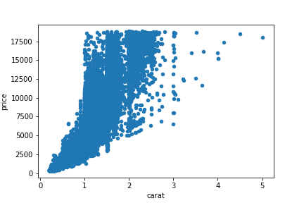
      Let’s plot these variables to check for the assumptions of a linear relationship being present and homoscedasticity of the data. We can use Pandas’s built in scatter plot method to complete this task.

      

      Based on the scatter plot, it appears that we are violating Pearson’s correlation assumption of homoscedasticity. For a more rigorous test, we can test the variances using the Levene’s test.

      stats.levene(df['carat'], df['price']) 

      Levene’s test for equal variances is significant, meaning we violate the assumption of homoscedasticity. Given that, the appropriate correlation test to use would be the Spearman Rank correlation test. For demonstration purposes, we will also conduct the Pearson correlation test.

      The Pandas Correlation Method

      To conduct the correlation test itself, we can use the .corr() method. This method conducts the correlation test between the variables and excludes all missing values. It can conduct the correlation test using a Pearson (the default method), Kendall, and Spearman method. Official documentation is here.

      df['carat'].corr(df['price'], method= 'spearman') 

      You can see that the two different methods of calculating the level of correlation between the variables produces different results. Both methods show a strong level of correlation between the carat of the diamond and the price of the diamond. Unfortunately, the built-in Pandas method does not provide a way to obtain the p-value for the correlation test. But fear not! There are other methods that are available to use.

      Pearson Correlation Method using scipy.stats.pearsonr()

      Scipy Stats is a great library for Python with many statistical tests available. Here is the full list of statistical tests available in this library. We will be using the pearsonr() method. First, we have to import this library!

      import scipy.stats as stats 

      Now let’s conduct the correlation test using the pearsonr() method for demonstration purposes and obtain both the correlation value and p-value. Unfortunately the output is not labeled, but it is printed in the ordered of (r value, p-value).

      stats.pearsonr(df['carat'], df['price']) 

      We see that the correlation is strong and significant between the size of the carat and the price of the diamond. Remember this is not the correct correlation test to use for our data as it violated the assumption of homoscedasticity. We should have conducted the correlation test using the Spearman Rank method or Kendall’s Tau-b.

      Spearman Rank Correlation Method using scipy.stats.spearmanr()

      Now let’s conduct the correlation test using the spearmanr() method and obtain both the correlation value and p-value. Given our data, this is a viable alternative correlation method to use.

      stats.spearmanr(df['carat'], df['price'])']) 

      (correlation= 0.96, pvalue= 0.0)

      We see that the correlation is strong and significant between the size of the carat and the price of the diamond.

      Kendall Tau-B Correlation Method using scipy.stats.kendalltau()

      Now let’s conduct the correlation test using the kendalltau() method and obtain both the correlation value and p-value. Given our data, this is a viable alternative correlation method to use. It is used less than Spearman Rank correlation, but this method handles ties in the data better.

      stats.kendalltau(df['carat'], df['price']) 

      (correlation= 0.83, pvalue= 0.0)

      Using this method, we see that there is still a strong correlation between the size of the carat and the price of the diamond.

      Correlation on Multiple Variables

      There will be times you will want to find the correlation values and p-values for multiple variables. It would be tiresome to repeat all the steps we just completed for all the variables of interest. Fear not! Below are custom functions that will save you time. You will have to decide if you want to use list-wise deletion or pair-wise deletion.

      List-wise deletion

      List-wise deletion keeps only the completed cases for all variables being tested at that time. Meaning, if testing 3 variables and they each have a different amount of completed cases (N), the smallest N of those 3 will be used for all the variables.

      This function conducts list-wise deletion, finds the Pearson, Spearman Rank, or Kendall’s Tau-b correlation values, and the significance of those. It also has the ability to export the results to a csv file. The correlation and p-values are printed in their own table. You need to import pandas and scipy.stats for this function to work.

      import pandas as pd import scipt.stats as stats def lwise_corr_pvalues(df, to_csv= False, file_name = None, method= None): df = df.dropna(how= 'any')._get_numeric_data() dfcols = pd.DataFrame(columns=df.columns) rvalues = dfcols.transpose().join(dfcols, how='outer') pvalues = dfcols.transpose().join(dfcols, how='outer') length = str(len(df)) if method == None: test = stats.pearsonr test_name = "Pearson" elif method == "spearman": test = stats.spearmanr test_name = "Spearman Rank" elif method == "kendall": test = stats.kendalltau test_name = "Kendall's Tau-b" for r in df.columns: for c in df.columns: rvalues[r][c] = round(test(df[r], df[c])[0], 4) for r in df.columns: for c in df.columns: pvalues[r][c] = format(test(df[r], df[c])[1], '.4f') if to_csv == False: print("Correlation test conducted using list-wise deletion", "\n", "Total observations used: ",length, "\n", "\n", f" Correlation Values", "\n", rvalues, "\n", "Significant Levels", "\n", pvalues) if to_csv == True: print("Correlation test conducted using list-wise deletion", "\n", "Total observations used: ",length, "\n", "\n", f" Correlation Values", "\n", rvalues, "\n", "Significant Levels", "\n", pvalues) file = open(file_name, 'a') file.write("Correlation test conducted using list-wise deletion" + "\n" + f" correlation values" + "\n") file.write("Total observations used: " + length + "\n") file.close() rvalues.to_csv(file_name, header= True, mode= 'a') file = open(file_name, 'a') file.write("p-values" + "\n") file.close() pvalues.to_csv(file_name, header= True, mode= 'a') 

      lwise_corr_pvalues(df[['carat', 'price', 'depth']]) 

      Correlation test conducted using list-wise deletion Total observations used: 53,940
      Pearson Correlation Values
      carat	price	depth
      carat	1	0.9216	0.0282
      price	0.9216	1	-0.0106
      depth	0.0282	-0.0106	1
      Significant Levels
      carat	price	depth
      carat	0.000	0.000	0.000
      price	0.000	0.000	0.0134
      depth	0.000	0.0134	0.000

      Pair-wise deletion

      Using pair-wise deletion when calculating correlations between multiple variables at a time will only remove the missing cases between the 2 variables being compare at that time. Meaning, each correlation value could be based off of a different N.

      If you want to run correlations using the pair-wise deletion method then use this custom function! It removes all missing values only for the 2 variables being compared at that time and reports the Pearson, Spearman Rank, or Kendall’s Tau-b correlation value, p-value, and number of observations used in the calculation. It also has the ability to export the results to a csv file. You have to import pandas, scipy.stats, and itertools for this to work.

      import pandas as pd import scipt.stats as stats import itertools def pwise_corr_pvalues(df, to_csv= False, file_name = None, method= None): correlations = <> pvalues = <> length = <> columns = df.columns.tolist() if method == None: test = stats.pearsonr test_name = "Pearson" elif method == "spearman": test = stats.spearmanr test_name = "Spearman Rank" elif method == "kendall": test = stats.kendalltau test_name = "Kendall's Tau-b" for col1, col2 in itertools.combinations(columns, 2): sub = df[[col1,col2]].dropna(how= "any") correlations[col1 + " " + "&" + " " + col2] = format(test(sub.loc[:, col1], sub.loc[:, col2])[0], '.4f') pvalues[col1 + " " + "&" + " " + col2] = format(test(sub.loc[:, col1], sub.loc[:, col2])[1], '.4f') length[col1 + " " + "&" + " " + col2] = len(df[[col1,col2]].dropna(how= "any")) corrs = pd.DataFrame.from_dict(correlations, orient= "index") corrs.columns = ["r value"] pvals = pd.DataFrame.from_dict(pvalues, orient= "index") pvals.columns = ["p-value"] l = pd.DataFrame.from_dict(length, orient= "index") l.columns = ["N"] results = corrs.join([pvals,l]) if to_csv == False: print(f" correlation", "\n", results) if to_csv == True: print(results) results.to_csv(file_name, header= True, mode = 'w', float_format='%.4f') 

      pwise_corr_pvalues(df[['carat', 'price', 'depth']]) 

      r value	p-value	N
      carat & price	0.9216	0.0000	53,940
      carat & depth	0.0282	0.0000	53,940
      price & depth	-0.0106	0.0134	53,940

      How to Video

      Источник

      Читайте также:  Php table not creating