Simple 1D Kernel Density Estimation
This example uses the KernelDensity class to demonstrate the principles of Kernel Density Estimation in one dimension.
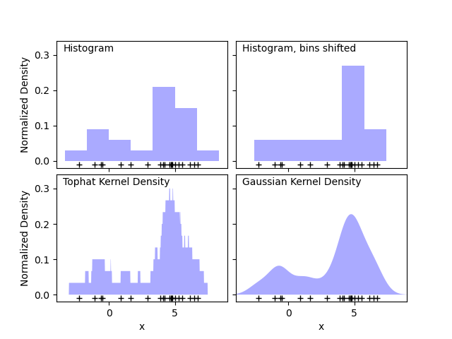
The first plot shows one of the problems with using histograms to visualize the density of points in 1D. Intuitively, a histogram can be thought of as a scheme in which a unit “block” is stacked above each point on a regular grid. As the top two panels show, however, the choice of gridding for these blocks can lead to wildly divergent ideas about the underlying shape of the density distribution. If we instead center each block on the point it represents, we get the estimate shown in the bottom left panel. This is a kernel density estimation with a “top hat” kernel. This idea can be generalized to other kernel shapes: the bottom-right panel of the first figure shows a Gaussian kernel density estimate over the same distribution.
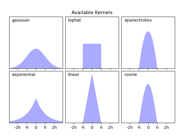
Scikit-learn implements efficient kernel density estimation using either a Ball Tree or KD Tree structure, through the KernelDensity estimator. The available kernels are shown in the second figure of this example.
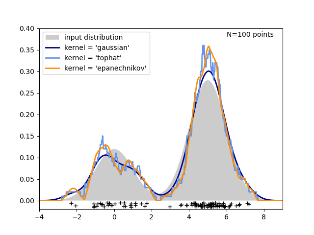
The third figure compares kernel density estimates for a distribution of 100 samples in 1 dimension. Though this example uses 1D distributions, kernel density estimation is easily and efficiently extensible to higher dimensions as well.
# Author: Jake Vanderplas # import matplotlib.pyplot as plt import numpy as np from scipy.stats import norm from sklearn.neighbors import KernelDensity # ---------------------------------------------------------------------- # Plot the progression of histograms to kernels np.random.seed(1) N = 20 X = np.concatenate( (np.random.normal(0, 1, int(0.3 * N)), np.random.normal(5, 1, int(0.7 * N))) )[:, np.newaxis] X_plot = np.linspace(-5, 10, 1000)[:, np.newaxis] bins = np.linspace(-5, 10, 10) fig, ax = plt.subplots(2, 2, sharex=True, sharey=True) fig.subplots_adjust(hspace=0.05, wspace=0.05) # histogram 1 ax[0, 0].hist(X[:, 0], bins=bins, fc="#AAAAFF", density=True) ax[0, 0].text(-3.5, 0.31, "Histogram") # histogram 2 ax[0, 1].hist(X[:, 0], bins=bins + 0.75, fc="#AAAAFF", density=True) ax[0, 1].text(-3.5, 0.31, "Histogram, bins shifted") # tophat KDE kde = KernelDensity(kernel="tophat", bandwidth=0.75).fit(X) log_dens = kde.score_samples(X_plot) ax[1, 0].fill(X_plot[:, 0], np.exp(log_dens), fc="#AAAAFF") ax[1, 0].text(-3.5, 0.31, "Tophat Kernel Density") # Gaussian KDE kde = KernelDensity(kernel="gaussian", bandwidth=0.75).fit(X) log_dens = kde.score_samples(X_plot) ax[1, 1].fill(X_plot[:, 0], np.exp(log_dens), fc="#AAAAFF") ax[1, 1].text(-3.5, 0.31, "Gaussian Kernel Density") for axi in ax.ravel(): axi.plot(X[:, 0], np.full(X.shape[0], -0.01), "+k") axi.set_xlim(-4, 9) axi.set_ylim(-0.02, 0.34) for axi in ax[:, 0]: axi.set_ylabel("Normalized Density") for axi in ax[1, :]: axi.set_xlabel("x") # ---------------------------------------------------------------------- # Plot all available kernels X_plot = np.linspace(-6, 6, 1000)[:, None] X_src = np.zeros((1, 1)) fig, ax = plt.subplots(2, 3, sharex=True, sharey=True) fig.subplots_adjust(left=0.05, right=0.95, hspace=0.05, wspace=0.05) def format_func(x, loc): if x == 0: return "0" elif x == 1: return "h" elif x == -1: return "-h" else: return "%ih" % x for i, kernel in enumerate( ["gaussian", "tophat", "epanechnikov", "exponential", "linear", "cosine"] ): axi = ax.ravel()[i] log_dens = KernelDensity(kernel=kernel).fit(X_src).score_samples(X_plot) axi.fill(X_plot[:, 0], np.exp(log_dens), "-k", fc="#AAAAFF") axi.text(-2.6, 0.95, kernel) axi.xaxis.set_major_formatter(plt.FuncFormatter(format_func)) axi.xaxis.set_major_locator(plt.MultipleLocator(1)) axi.yaxis.set_major_locator(plt.NullLocator()) axi.set_ylim(0, 1.05) axi.set_xlim(-2.9, 2.9) ax[0, 1].set_title("Available Kernels") # ---------------------------------------------------------------------- # Plot a 1D density example N = 100 np.random.seed(1) X = np.concatenate( (np.random.normal(0, 1, int(0.3 * N)), np.random.normal(5, 1, int(0.7 * N))) )[:, np.newaxis] X_plot = np.linspace(-5, 10, 1000)[:, np.newaxis] true_dens = 0.3 * norm(0, 1).pdf(X_plot[:, 0]) + 0.7 * norm(5, 1).pdf(X_plot[:, 0]) fig, ax = plt.subplots() ax.fill(X_plot[:, 0], true_dens, fc="black", alpha=0.2, label="input distribution") colors = ["navy", "cornflowerblue", "darkorange"] kernels = ["gaussian", "tophat", "epanechnikov"] lw = 2 for color, kernel in zip(colors, kernels): kde = KernelDensity(kernel=kernel, bandwidth=0.5).fit(X) log_dens = kde.score_samples(X_plot) ax.plot( X_plot[:, 0], np.exp(log_dens), color=color, lw=lw, linestyle="-", label="kernel = ' '".format(kernel), ) ax.text(6, 0.38, "N= points".format(N)) ax.legend(loc="upper left") ax.plot(X[:, 0], -0.005 - 0.01 * np.random.random(X.shape[0]), "+k") ax.set_xlim(-4, 9) ax.set_ylim(-0.02, 0.4) plt.show() Total running time of the script: ( 0 minutes 0.615 seconds)
sklearn.neighbors .KernelDensity
class sklearn.neighbors. KernelDensity ( * , bandwidth = 1.0 , algorithm = ‘auto’ , kernel = ‘gaussian’ , metric = ‘euclidean’ , atol = 0 , rtol = 0 , breadth_first = True , leaf_size = 40 , metric_params = None ) [source] 
Kernel Density Estimation.
Parameters : bandwidth float or , default=1.0
The bandwidth of the kernel. If bandwidth is a float, it defines the bandwidth of the kernel. If bandwidth is a string, one of the estimation methods is implemented.
The tree algorithm to use.
metric str, default=’euclidean’
Metric to use for distance computation. See the documentation of scipy.spatial.distance and the metrics listed in distance_metrics for valid metric values.
Not all metrics are valid with all algorithms: refer to the documentation of BallTree and KDTree . Note that the normalization of the density output is correct only for the Euclidean distance metric.
atol float, default=0
The desired absolute tolerance of the result. A larger tolerance will generally lead to faster execution.
rtol float, default=0
The desired relative tolerance of the result. A larger tolerance will generally lead to faster execution.
breadth_first bool, default=True
If true (default), use a breadth-first approach to the problem. Otherwise use a depth-first approach.
leaf_size int, default=40
Specify the leaf size of the underlying tree. See BallTree or KDTree for details.
metric_params dict, default=None
Additional parameters to be passed to the tree for use with the metric. For more information, see the documentation of BallTree or KDTree .
Attributes : n_features_in_ int
Number of features seen during fit .
The tree algorithm for fast generalized N-point problems.
feature_names_in_ ndarray of shape ( n_features_in_ ,)
Names of features seen during fit . Defined only when X has feature names that are all strings.
bandwidth_ float
Value of the bandwidth, given directly by the bandwidth parameter or estimated using the ‘scott’ or ‘silverman’ method.
K-dimensional tree for fast generalized N-point problems.
Ball tree for fast generalized N-point problems.
Compute a gaussian kernel density estimate with a fixed bandwidth.
>>> from sklearn.neighbors import KernelDensity >>> import numpy as np >>> rng = np.random.RandomState(42) >>> X = rng.random_sample((100, 3)) >>> kde = KernelDensity(kernel='gaussian', bandwidth=0.5).fit(X) >>> log_density = kde.score_samples(X[:3]) >>> log_density array([-1.52955942, -1.51462041, -1.60244657])
Fit the Kernel Density model on the data.
Get metadata routing of this object.
Get parameters for this estimator.
Generate random samples from the model.
Compute the total log-likelihood under the model.
Compute the log-likelihood of each sample under the model.
Request metadata passed to the fit method.
Set the parameters of this estimator.
Fit the Kernel Density model on the data.
Parameters : X array-like of shape (n_samples, n_features)
List of n_features-dimensional data points. Each row corresponds to a single data point.
Ignored. This parameter exists only for compatibility with Pipeline .
sample_weight array-like of shape (n_samples,), default=None
List of sample weights attached to the data X.
Returns the instance itself.
Get metadata routing of this object.
Please check User Guide on how the routing mechanism works.
Returns : routing MetadataRequest
A MetadataRequest encapsulating routing information.
Get parameters for this estimator.
Parameters : deep bool, default=True
If True, will return the parameters for this estimator and contained subobjects that are estimators.
Returns : params dict
Parameter names mapped to their values.
sample ( n_samples = 1 , random_state = None ) [source] 
Generate random samples from the model.
Currently, this is implemented only for gaussian and tophat kernels.
Parameters : n_samples int, default=1
Number of samples to generate.
random_state int, RandomState instance or None, default=None
Determines random number generation used to generate random samples. Pass an int for reproducible results across multiple function calls. See Glossary .
Returns : X array-like of shape (n_samples, n_features)
Compute the total log-likelihood under the model.
Parameters : X array-like of shape (n_samples, n_features)
List of n_features-dimensional data points. Each row corresponds to a single data point.
Ignored. This parameter exists only for compatibility with Pipeline .
Returns : logprob float
Total log-likelihood of the data in X. This is normalized to be a probability density, so the value will be low for high-dimensional data.
Compute the log-likelihood of each sample under the model.
Parameters : X array-like of shape (n_samples, n_features)
An array of points to query. Last dimension should match dimension of training data (n_features).
Returns : density ndarray of shape (n_samples,)
Log-likelihood of each sample in X . These are normalized to be probability densities, so values will be low for high-dimensional data.
Request metadata passed to the fit method.
Note that this method is only relevant if enable_metadata_routing=True (see sklearn.set_config ). Please see User Guide on how the routing mechanism works.
The options for each parameter are:
- True : metadata is requested, and passed to fit if provided. The request is ignored if metadata is not provided.
- False : metadata is not requested and the meta-estimator will not pass it to fit .
- None : metadata is not requested, and the meta-estimator will raise an error if the user provides it.
- str : metadata should be passed to the meta-estimator with this given alias instead of the original name.
The default ( sklearn.utils.metadata_routing.UNCHANGED ) retains the existing request. This allows you to change the request for some parameters and not others.
This method is only relevant if this estimator is used as a sub-estimator of a meta-estimator, e.g. used inside a pipeline.Pipeline . Otherwise it has no effect.
Parameters : sample_weight str, True, False, or None, default=sklearn.utils.metadata_routing.UNCHANGED
Metadata routing for sample_weight parameter in fit .
Returns : self object
Set the parameters of this estimator.
The method works on simple estimators as well as on nested objects (such as Pipeline ). The latter have parameters of the form __ so that it’s possible to update each component of a nested object.
Parameters : **params dict
Returns : self estimator instance


