Heat equation in 2D#
This tutorial solves the stationary heat equation in 2D. The example is taken from the pyGIMLi paper (https://cg17.pygimli.org).
import pygimli as pg import pygimli.meshtools as mt
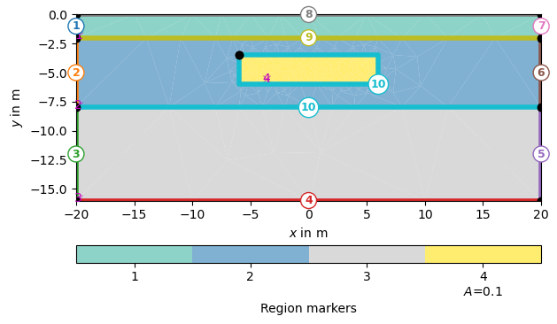
Create geometry definition for the modelling domain.
world = mt.createWorld(start=[-20, 0], end=[20, -16], layers=[-2, -8], worldMarker=False) # Create a heterogeneous block block = mt.createRectangle(start=[-6, -3.5], end=[6, -6.0], marker=4, boundaryMarker=10, area=0.1) # Merge geometrical entities geom = world + block pg.show(geom, markers=True)
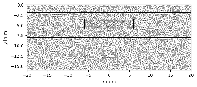
Create a mesh from based on the geometry definition. When calling the pg.meshtools.createMesh() function, a quality parameter can be forwarded to Triangle, which prescribes the minimum angle allowed in the final mesh. For a tutorial on the quality of the mesh please refer to : Mesh quality inspection [1] [1]: https://www.pygimli.org/_tutorials_auto/1_basics/plot_6-mesh-quality-inspection.html#sphx-glr-tutorials-auto-1-basics-plot-6-mesh-quality-inspection-py Note: Incrementing quality increases computer time, take precaution with quality values over 33.
mesh = mt.createMesh(geom, quality=33, area=0.2, smooth=[1, 10]) pg.show(mesh)
Call pygimli.solver.solveFiniteElements() to solve the heat diffusion equation \(\nabla\cdot(a\nabla T)=0\) with \(T(bottom)=0\) (boundary marker 8) and \(T(top)=1\) (boundary marker 4), where \(a\) is the thermal diffusivity and \(T\) is the temperature distribution. We assign thermal diffusivities to the four # regions using their marker numbers in a dictionary (a) and the fixed temperatures at the boundaries using Dirichlet boundary conditions with the respective markers in another dictionary (bc)
T = pg.solver.solveFiniteElements(mesh, a=1: 1.0, 2: 2.0, 3: 3.0, 4:0.1>, bc='Dirichlet': 8: 1.0, 4: 0.0>>, verbose=True) ax, _ = pg.show(mesh, data=T, label='Temperature $T$', cMap="hot_r", nCols=8, contourLines=False) pg.show(geom, ax=ax, fillRegion=False)
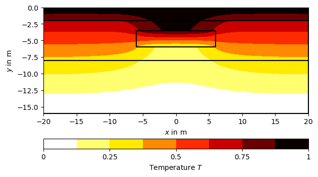
Mesh: Mesh: Nodes: 3011 Cells: 5832 Boundaries: 8842 Assembling time: 0.042252237 Solving time: 0.483438497 (, None)
Solving 2D Heat Equation Numerically using Python
When I was in college studying physics a few years ago, I remember there was a task to solve heat equation analytically for some simple problems. In the next semester we learned about numerical methods to solve some partial differential equations (PDEs) in general. It’s really interesting to see how we could solve them numerically and visualize the solutions as a heat map, and it’s really cool (pun intended). I also remember, in the previous semester we learned C programming language, so it was natural for us to solve PDEs numerically using C although some students were struggling with C and not with solving the PDE itself. If I had known how to code in Python back then, I would’ve used it instead of C (I am not saying C is bad though). Here, I am going to show how we can solve 2D heat equation numerically and see how easy it is to “translate” the equations into Python code.
Before we do the Python code, let’s talk about the heat equation and finite-difference method. Heat equation is basically a partial differential equation, it is
If we want to solve it in 2D (Cartesian), we can write the heat equation above like this
where u is the quantity that we want to know, t is for temporal variable, x and y are for spatial variables, and α is diffusivity constant. So basically we want to find the solution u everywhere in x and y, and over time t.
Now let’s see the finite-difference method (FDM) in a nutshell. Finite-difference method is a numerical method for solving differential equations by approximating derivative with finite differences. Remember that the definition of derivative is
In finite-difference method, we approximate it and remove the limit. So, instead of using differential and limit symbol, we use delta symbol which is the finite difference. Note that this is oversimplified, because we have to use Taylor series expansion and derive it from there by assuming some terms to be sufficiently small, but we get the rough idea behind this method.
In finite-difference method, we are going to “discretize” the spatial domain and the time interval x, y, and t. We can write it like this
As we can see, i, j, and k are the steps for each difference for x, y, and t respectively. What we want is the solution u, which is
Note that k is superscript to denote time step for u. We can write the heat equation above using finite-difference method like this
If we arrange the equation above by taking Δx = Δy, we get this final equation
We can use this stencil to remember the equation above (look at subscripts i, j for spatial steps and superscript k for the time step)
We use explicit method to get the solution for the heat equation, so it will be numerically stable whenever
Everything is ready. Now we can solve the original heat equation approximated by algebraic equation above, which is computer-friendly. For an exercise problem, let’s suppose a thin square plate with the side of 50 unit length. The temperature everywhere inside the plate is originally 0 degree (at t = 0), let’s see the diagram below (this is not realistic, but it’s good for exercise)
For our model, let’s take Δx = 1 and α = 2.0. Now we can use Python code to solve this problem numerically to see the temperature everywhere (denoted by i and j) and over time (denoted by k). Let’s first import all of the necessary libraries, and then set up the boundary and initial conditions.
Cool isn’t it? By the way, you can try the code above using this Python Online Compiler https://repl.it/languages/python3, make sure you change the max_iter_time to 50 before you run the code to make the iteration result faster.
Okay, we have the code now, let’s play with something more interesting, let’s set all of the boundary conditions to 0, and then randomize the initial condition for the interior grid.
Python is relatively easy to learn for beginners compared to other programming languages. I would recommend to use Python for solving computational problems like we’ve done here, at least for prototyping because it has really powerful numerical and scientific libraries. The community is also growing bigger and bigger, and that can make things easier to Google when we’re stuck with it. Python may not be as fast as C or C++, but using Python we can focus more on the problem solving itself rather than the language, of course we still need to know the Python syntax and its simple array manipulation to some degree, but once we get it, it will be really powerful.
Level Up Coding
Thanks for being a part of our community! Level Up is transforming tech recruiting. Find your perfect job at the best companies.
Solving 2D Heat Equation…

where u is the quantity that we want to know, t is for temporal variable, x and y are for spatial variables, and α is diffusivity constant. So basically we want to find the solution u everywhere in x and y, and over time t. We can write the heat equation above using finite-difference method like this:


where \(\gamma = \alpha \frac>>>\) We use explicit method to get the solution for the heat equation, so it will be numerically stable whenever \(\Delta t \leq \frac>>>\) Everything is ready. Now we can solve the original heat equation approximated by algebraic equation above, which is computer-friendly. Let’s suppose a thin square plate with the side of 50 unit length. The temperature everywhere inside the plate is originally 0 degree (at t = 0), let’s see the diagram below:

For our model, let’s take Δx = 1 and α = 2.0.
Now we can use Python code to solve this problem numerically to see the temperature everywhere (denoted by i and j) and over time (denoted by k). Let’s first import all of the necessary libraries, and then set up the boundary and initial conditions.
import numpy as np import matplotlib.pyplot as plt import matplotlib.animation as animation from matplotlib.animation import FuncAnimation print("2D heat equation solver") plate_length = 50 max_iter_time = 750 alpha = 2 delta_x = 1 delta_t = (delta_x ** 2)/(4 * alpha) gamma = (alpha * delta_t) / (delta_x ** 2) # Initialize solution: the grid of u(k, i, j) u = np.empty((max_iter_time, plate_length, plate_length)) # Initial condition everywhere inside the grid u_initial = 0 # Boundary conditions u_top = 100.0 u_left = 0.0 u_bottom = 0.0 u_right = 0.0 # Set the initial condition u.fill(u_initial) # Set the boundary conditions u[:, (plate_length-1):, :] = u_top u[:, :, :1] = u_left u[:, :1, 1:] = u_bottom u[:, :, (plate_length-1):] = u_right We’ve set up the initial and boundary conditions, let’s write the calculation function based on finite-difference method that we’ve derived above.
def calculate(u): for k in range(0, max_iter_time-1, 1): for i in range(1, plate_length-1, delta_x): for j in range(1, plate_length-1, delta_x): u[k + 1, i, j] = gamma * (u[k][i+1][j] + u[k][i-1][j] + u[k][i][j+1] + u[k][i][j-1] - 4*u[k][i][j]) + u[k][i][j] return u
Let’s prepare the plot function so we can visualize the solution (for each k) as a heat map. We use Matplotlib library, it’s easy to use.
def plotheatmap(u_k, k): # Clear the current plot figure plt.clf() plt.title(f"Temperature at t = unit time") plt.xlabel("x") plt.ylabel("y") # This is to plot u_k (u at time-step k) plt.pcolormesh(u_k, cmap=plt.cm.jet, vmin=0, vmax=100) plt.colorbar() return plt One more thing that we need is to animate the result because we want to see the temperature points inside the plate change over time. So let’s create the function to animate the solution.
def animate(k): plotheatmap(u[k], k) anim = animation.FuncAnimation(plt.figure(), animate, interval=1, frames=max_iter_time, repeat=False) anim.save("heat_equation_solution.gif")