matplotlib.pyplot.plot#
The coordinates of the points or line nodes are given by x, y.
The optional parameter fmt is a convenient way for defining basic formatting like color, marker and linestyle. It’s a shortcut string notation described in the Notes section below.
>>> plot(x, y) # plot x and y using default line style and color >>> plot(x, y, 'bo') # plot x and y using blue circle markers >>> plot(y) # plot y using x as index array 0..N-1 >>> plot(y, 'r+') # ditto, but with red plusses
You can use Line2D properties as keyword arguments for more control on the appearance. Line properties and fmt can be mixed. The following two calls yield identical results:
>>> plot(x, y, 'go--', linewidth=2, markersize=12) >>> plot(x, y, color='green', marker='o', linestyle='dashed', . linewidth=2, markersize=12)
When conflicting with fmt, keyword arguments take precedence.
Plotting labelled data
There’s a convenient way for plotting objects with labelled data (i.e. data that can be accessed by index obj[‘y’] ). Instead of giving the data in x and y, you can provide the object in the data parameter and just give the labels for x and y:
>>> plot('xlabel', 'ylabel', data=obj)
All indexable objects are supported. This could e.g. be a dict , a pandas.DataFrame or a structured numpy array.
Plotting multiple sets of data
There are various ways to plot multiple sets of data.
- The most straight forward way is just to call plot multiple times. Example:
>>> plot(x1, y1, 'bo') >>> plot(x2, y2, 'go')
>>> x = [1, 2, 3] >>> y = np.array([[1, 2], [3, 4], [5, 6]]) >>> plot(x, y)
>>> for col in range(y.shape[1]): . plot(x, y[:, col])
By default, each line is assigned a different style specified by a ‘style cycle’. The fmt and line property parameters are only necessary if you want explicit deviations from these defaults. Alternatively, you can also change the style cycle using rcParams[«axes.prop_cycle»] (default: cycler(‘color’, [‘#1f77b4’, ‘#ff7f0e’, ‘#2ca02c’, ‘#d62728’, ‘#9467bd’, ‘#8c564b’, ‘#e377c2’, ‘#7f7f7f’, ‘#bcbd22’, ‘#17becf’]) ).
Parameters : x, y array-like or scalar
The horizontal / vertical coordinates of the data points. x values are optional and default to range(len(y)) .
Commonly, these parameters are 1D arrays.
They can also be scalars, or two-dimensional (in that case, the columns represent separate data sets).
These arguments cannot be passed as keywords.
fmt str, optional
A format string, e.g. ‘ro’ for red circles. See the Notes section for a full description of the format strings.
Format strings are just an abbreviation for quickly setting basic line properties. All of these and more can also be controlled by keyword arguments.
This argument cannot be passed as keyword.
data indexable object, optional
An object with labelled data. If given, provide the label names to plot in x and y.
Technically there’s a slight ambiguity in calls where the second label is a valid fmt. plot(‘n’, ‘o’, data=obj) could be plt(x, y) or plt(y, fmt) . In such cases, the former interpretation is chosen, but a warning is issued. You may suppress the warning by adding an empty format string plot(‘n’, ‘o’, », data=obj) .
A list of lines representing the plotted data.
Other Parameters : scalex, scaley bool, default: True
These parameters determine if the view limits are adapted to the data limits. The values are passed on to autoscale_view .
**kwargs Line2D properties, optional
kwargs are used to specify properties like a line label (for auto legends), linewidth, antialiasing, marker face color. Example:
>>> plot([1, 2, 3], [1, 2, 3], 'go-', label='line 1', linewidth=2) >>> plot([1, 2, 3], [1, 4, 9], 'rs', label='line 2')
If you specify multiple lines with one plot call, the kwargs apply to all those lines. In case the label object is iterable, each element is used as labels for each set of data.
Here is a list of available Line2D properties:
a filter function, which takes a (m, n, 3) float array and a dpi value, and returns a (m, n, 3) array and two offsets from the bottom left corner of the image
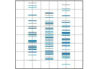
Plot types#
Overview of many common plotting commands in Matplotlib.
Note that we have stripped all labels, but they are present by default. See the gallery for many more examples and the tutorials page for longer examples.
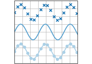
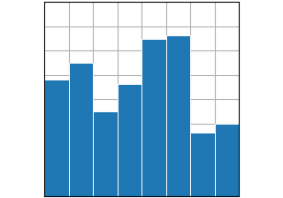
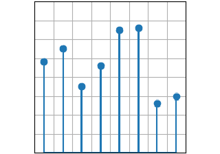
Basic#
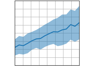
Basic plot types, usually y versus x.

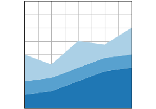
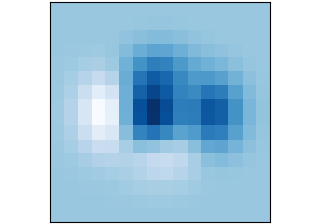
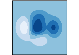
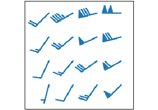
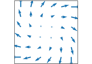
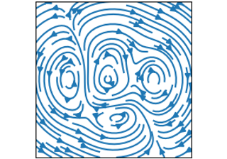
Plots of arrays and fields#
Plotting for arrays of data Z(x, y) and fields U(x, y), V(x, y) .

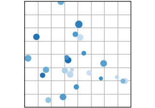
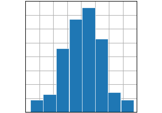
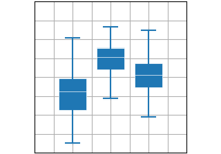
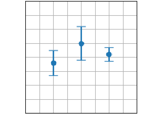
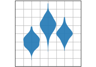
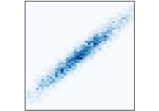
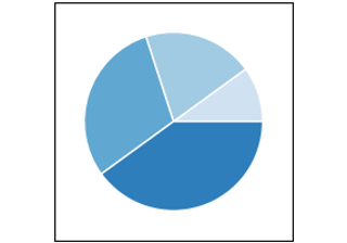
Statistics plots#
Plots for statistical analysis.
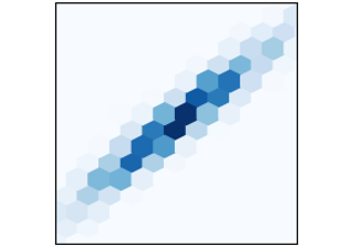
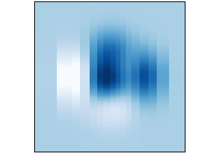
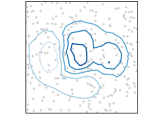
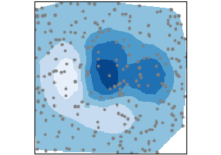
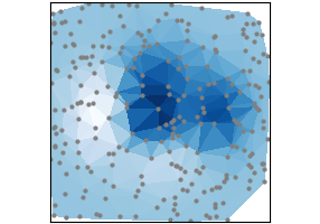
Unstructured coordinates#
Sometimes we collect data z at coordinates (x,y) and want to visualize as a contour. Instead of gridding the data and then using contour , we can use a triangulation algorithm and fill the triangles.

3D#
3D plots using the mpl_toolkits.mplot3d library.