DataTechNotes
We use Boston house-price dataset as regression dataset in this tutorial. After loading the dataset, first, we’ll separate data into x and y parts.
boston = load_boston() x, y = boston.data, boston.target
Then we’ll split it into train and test parts. Here, we’ll extract 15 percent of the data as a test.
xtrain, xtest, ytrain, ytest=train_test_split(x, y, random_state=12, test_size=0.15)
We can define the model with its default parameters or set the new parameter values.
# with new parameters gbr = GradientBoostingRegressor(n_estimators=600, max_depth=5, learning_rate=0.01, min_samples_split=3) # with default parameters gbr = GradientBoostingRegressor()
print(gbr) GradientBoostingRegressor(alpha=0.9, criterion='friedman_mse', init=None, learning_rate=0.1, loss='ls', max_depth=3, max_features=None, max_leaf_nodes=None, min_impurity_decrease=0.0, min_impurity_split=None, min_samples_leaf=1, min_samples_split=2, min_weight_fraction_leaf=0.0, n_estimators=100, presort='auto', random_state=None, subsample=1.0, verbose=0, warm_start=False)
Next, we’ll fit the model with train data.
Predicting test data and visualizing the result
We can predict the test data and check the error rate as a following.
ypred = gbr.predict(xtest) mse = mean_squared_error(ytest,ypred)
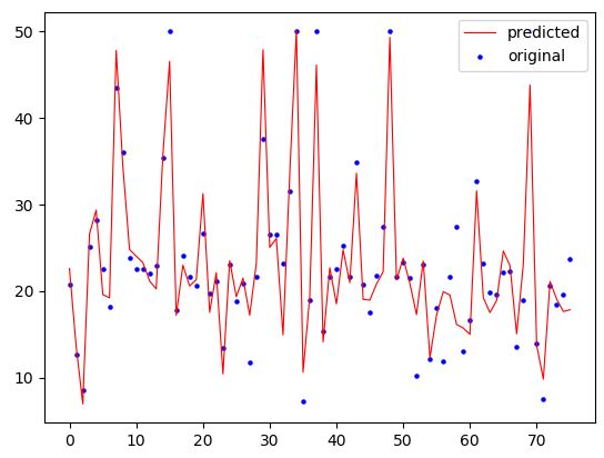
Finally, we’ll visualize the original and predicted values in a plot.
x_ax = range(len(ytest)) plt.scatter(x_ax, ytest, s=5, color="blue", label="original") plt.plot(x_ax, ypred, lw=0.8, color="red", label="predicted") plt.legend() plt.show()
In this post, we’ve briefly learned how to use Gradient Boosting Regressor to predict regression data in Python. Thank you for reading!
The full source code is listed below.
from sklearn.ensemble import GradientBoostingRegressor from sklearn.datasets import load_boston from sklearn.model_selection import train_test_split from sklearn.metrics import mean_squared_error import matplotlib.pyplot as plt boston = load_boston() x, y = boston.data, boston.target xtrain, xtest, ytrain, ytest=train_test_split(x, y, random_state=12, test_size=0.15) # with new parameters gbr = GradientBoostingRegressor(n_estimators=600, max_depth=5, learning_rate=0.01, min_samples_split=3) # with default parameters gbr = GradientBoostingRegressor() gbr.fit(xtrain, ytrain) ypred = gbr.predict(xtest) mse = mean_squared_error(ytest,ypred) print("MSE: %.2f" % mse) x_ax = range(len(ytest)) plt.scatter(x_ax, ytest, s=5, color="blue", label="original") plt.plot(x_ax, ypred, lw=0.8, color="red", label="predicted") plt.legend() plt.show()
Gradient Boosting regression
This example demonstrates Gradient Boosting to produce a predictive model from an ensemble of weak predictive models. Gradient boosting can be used for regression and classification problems. Here, we will train a model to tackle a diabetes regression task. We will obtain the results from GradientBoostingRegressor with least squares loss and 500 regression trees of depth 4.
Note: For larger datasets (n_samples >= 10000), please refer to HistGradientBoostingRegressor .
# Author: Peter Prettenhofer # Maria Telenczuk # Katrina Ni # # License: BSD 3 clause import matplotlib.pyplot as plt import numpy as np from sklearn import datasets, ensemble from sklearn.inspection import permutation_importance from sklearn.metrics import mean_squared_error from sklearn.model_selection import train_test_split Load the data
First we need to load the data.
diabetes = datasets.load_diabetes() X, y = diabetes.data, diabetes.target
Data preprocessing
Next, we will split our dataset to use 90% for training and leave the rest for testing. We will also set the regression model parameters. You can play with these parameters to see how the results change.
n_estimators : the number of boosting stages that will be performed. Later, we will plot deviance against boosting iterations.
max_depth : limits the number of nodes in the tree. The best value depends on the interaction of the input variables.
min_samples_split : the minimum number of samples required to split an internal node.
learning_rate : how much the contribution of each tree will shrink.
loss : loss function to optimize. The least squares function is used in this case however, there are many other options (see GradientBoostingRegressor ).
X_train, X_test, y_train, y_test = train_test_split( X, y, test_size=0.1, random_state=13 ) params = "n_estimators": 500, "max_depth": 4, "min_samples_split": 5, "learning_rate": 0.01, "loss": "squared_error", >
Fit regression model
Now we will initiate the gradient boosting regressors and fit it with our training data. Let’s also look and the mean squared error on the test data.
reg = ensemble.GradientBoostingRegressor(**params) reg.fit(X_train, y_train) mse = mean_squared_error(y_test, reg.predict(X_test)) print("The mean squared error (MSE) on test set: ".format(mse))
The mean squared error (MSE) on test set: 3025.7877
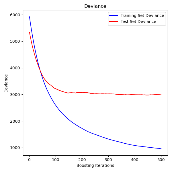
Plot training deviance
Finally, we will visualize the results. To do that we will first compute the test set deviance and then plot it against boosting iterations.
test_score = np.zeros((params["n_estimators"],), dtype=np.float64) for i, y_pred in enumerate(reg.staged_predict(X_test)): test_score[i] = mean_squared_error(y_test, y_pred) fig = plt.figure(figsize=(6, 6)) plt.subplot(1, 1, 1) plt.title("Deviance") plt.plot( np.arange(params["n_estimators"]) + 1, reg.train_score_, "b-", label="Training Set Deviance", ) plt.plot( np.arange(params["n_estimators"]) + 1, test_score, "r-", label="Test Set Deviance" ) plt.legend(loc="upper right") plt.xlabel("Boosting Iterations") plt.ylabel("Deviance") fig.tight_layout() plt.show()
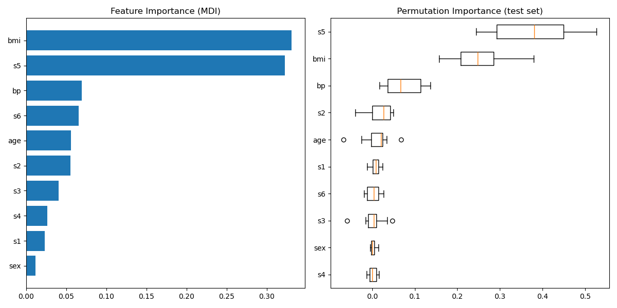
Plot feature importance
Careful, impurity-based feature importances can be misleading for high cardinality features (many unique values). As an alternative, the permutation importances of reg can be computed on a held out test set. See Permutation feature importance for more details.
For this example, the impurity-based and permutation methods identify the same 2 strongly predictive features but not in the same order. The third most predictive feature, “bp”, is also the same for the 2 methods. The remaining features are less predictive and the error bars of the permutation plot show that they overlap with 0.
feature_importance = reg.feature_importances_ sorted_idx = np.argsort(feature_importance) pos = np.arange(sorted_idx.shape[0]) + 0.5 fig = plt.figure(figsize=(12, 6)) plt.subplot(1, 2, 1) plt.barh(pos, feature_importance[sorted_idx], align="center") plt.yticks(pos, np.array(diabetes.feature_names)[sorted_idx]) plt.title("Feature Importance (MDI)") result = permutation_importance( reg, X_test, y_test, n_repeats=10, random_state=42, n_jobs=2 ) sorted_idx = result.importances_mean.argsort() plt.subplot(1, 2, 2) plt.boxplot( result.importances[sorted_idx].T, vert=False, labels=np.array(diabetes.feature_names)[sorted_idx], ) plt.title("Permutation Importance (test set)") fig.tight_layout() plt.show()
Total running time of the script: ( 0 minutes 1.250 seconds)
Gradient Boosting Regression in Python


In this post, we will take a look at gradient boosting for regression. Gradient boosting simply makes sequential models that try to explain any examples that had not been explained by previously models. This approach makes gradient boosting superior to AdaBoost.
Regression trees are mostly commonly teamed with boosting. There are some additional hyperparameters that need to be set which includes the following
We will deal with each of these when it is appropriate. Our goal in this post is to predict the amount of weight loss in cancer patients based on the independent variables. This is the process we will follow to achieve this.
- Data preparation
- Baseline decision tree model
- Hyperparameter tuning
- Gradient boosting model development
Below is some initial code
from sklearn.ensemble import GradientBoostingRegressor from sklearn import tree from sklearn.model_selection import GridSearchCV import numpy as np from pydataset import data import pandas as pd from sklearn.model_selection import cross_val_score from sklearn.model_selection import KFold
Data Preparation
The data preparation is not that difficult in this situation. We simply need to load the dataset in an object and remove any missing values. Then we separate the independent and dependent variables into separate datasets. The code is below.
df=data('cancer').dropna() X=df[['time','sex','ph.karno','pat.karno','status','meal.cal']] y=df['wt.loss'] We can now move to creating our baseline model.
Baseline Model
The purpose of the baseline model is to have something to compare our gradient boosting model to. Therefore, all we will do here is create several regression trees. The difference between the regression trees will be the max depth. The max depth has to with the number of nodes python can make to try to purify the classification. We will then decide which tree is best based on the mean squared error.
The first thing we need to do is set the arguments for the cross-validation. Cross validating the results helps to check the accuracy of the results. The rest of the code requires the use of for loops and if statements that cannot be reexplained in this post. Below is the code with the output.
crossvalidation=KFold(n_splits=10,shuffle=True,random_state=1)
for depth in range (1,10): tree_regressor=tree.DecisionTreeRegressor(max_depth=depth,random_state=1) if tree_regressor.fit(X,y).tree_.max_depth1 -193.55304528235052 2 -176.27520747356175 3 -209.2846723461564 4 -218.80238479654003 5 -222.4393459885871 6 -249.95330609042858 7 -286.76842138165705 8 -294.0290706405905 9 -287.39016236497804You can see that a max depth of 2 had the lowest amount of error. Therefore, our baseline model has a mean squared error of 176. We need to improve on this in order to say that our gradient boosting model is superior.
However, before we create our gradient boosting model. we need to tune the hyperparameters of the algorithm.
Hyperparameter Tuning
Hyperparameter tuning has to with setting the value of parameters that the algorithm cannot learn on its own. As such, these are constants that you set as the researcher. The problem is that you are not any better at knowing where to set these values than the computer. Therefore, the process that is commonly used is to have the algorithm use several combinations of values until it finds the values that are best for the model/. Having said this, there are several hyperparameters we need to tune, and they are as follows.
The number of estimators is show many trees to create. The more trees the more likely to overfit. The learning rate is the weight that each tree has on the final prediction. Subsample is the proportion of the sample to use. Max depth was explained previously.
What we will do now is make an instance of the GradientBoostingRegressor. Next, we will create our grid with the various values for the hyperparameters. We will then take this grid and place it inside GridSearchCV function so that we can prepare to run our model. There are some arguments that need to be set inside the GridSearchCV function such as estimator, grid, cv, etc. Below is the code.
GBR=GradientBoostingRegressor() search_grid= search=GridSearchCV(estimator=GBR,param_grid=search_grid,scoring='neg_mean_squared_error',n_jobs=1,cv=crossvalidation)We can now run the code and determine the best combination of hyperparameters and how well the model did base on the means squared error metric. Below is the code and the output.
search.fit(X,y) search.best_params_ Out[13]: search.best_score_ Out[14]: -160.51398257591643The hyperparameter results speak for themselves. With this tuning we can see that the mean squared error is lower than with the baseline model. We can now move to the final step of taking these hyperparameter settings and see how they do on the dataset. The results should be almost the same.
Gradient Boosting Model Development
Below is the code and the output for the tuned gradient boosting model
GBR2=GradientBoostingRegressor(n_estimators=500,learning_rate=0.01,subsample=.5,max_depth=1,random_state=1) score=np.mean(cross_val_score(GBR2,X,y,scoring='neg_mean_squared_error',cv=crossvalidation,n_jobs=1)) score Out[18]: -160.77842893572068These results were to be expected. The gradient boosting model has a better performance than the baseline regression tree model.
In this post, we looked at how to use gradient boosting to improve a regression tree. By creating multiple models. Gradient boosting will almost certainly have a better performance than other type of algorithms that rely on only one model.