Feature importance python примеры

Feature importances with a forest of trees¶

This example shows the use of a forest of trees to evaluate the importance of features on an artificial classification task. The blue bars are the feature importances of the forest, along with their inter-trees variability represented by the error bars.

As expected, the plot suggests that 3 features are informative, while the remaining are not.

import matplotlib.pyplot as plt 

Data generation and model fitting¶

We generate a synthetic dataset with only 3 informative features. We will explicitly not shuffle the dataset to ensure that the informative features will correspond to the three first columns of X. In addition, we will split our dataset into training and testing subsets.

from sklearn.datasets import make_classification from sklearn.model_selection import train_test_split X, y = make_classification( n_samples=1000, n_features=10, n_informative=3, n_redundant=0, n_repeated=0, n_classes=2, random_state=0, shuffle=False, ) X_train, X_test, y_train, y_test = train_test_split(X, y, stratify=y, random_state=42) 

A random forest classifier will be fitted to compute the feature importances.

from sklearn.ensemble import RandomForestClassifier feature_names = [f"feature i>" for i in range(X.shape[1])] forest = RandomForestClassifier(random_state=0) forest.fit(X_train, y_train) 

RandomForestClassifier(random_state=0)

In a Jupyter environment, please rerun this cell to show the HTML representation or trust the notebook.
On GitHub, the HTML representation is unable to render, please try loading this page with nbviewer.org.

RandomForestClassifier(random_state=0)

Feature importance based on mean decrease in impurity¶

Feature importances are provided by the fitted attribute feature_importances_ and they are computed as the mean and standard deviation of accumulation of the impurity decrease within each tree.

Impurity-based feature importances can be misleading for high cardinality features (many unique values). See Permutation feature importance as an alternative below.

import time import numpy as np start_time = time.time() importances = forest.feature_importances_ std = np.std([tree.feature_importances_ for tree in forest.estimators_], axis=0) elapsed_time = time.time() - start_time print(f"Elapsed time to compute the importances: elapsed_time:.3f> seconds") 

Elapsed time to compute the importances: 0.007 seconds

Let’s plot the impurity-based importance.

import pandas as pd forest_importances = pd.Series(importances, index=feature_names) fig, ax = plt.subplots() forest_importances.plot.bar(yerr=std, ax=ax) ax.set_title("Feature importances using MDI") ax.set_ylabel("Mean decrease in impurity") fig.tight_layout() 

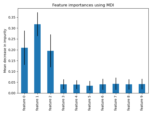
We observe that, as expected, the three first features are found important.

Feature importance based on feature permutation¶

Permutation feature importance overcomes limitations of the impurity-based feature importance: they do not have a bias toward high-cardinality features and can be computed on a left-out test set.

from sklearn.inspection import permutation_importance start_time = time.time() result = permutation_importance( forest, X_test, y_test, n_repeats=10, random_state=42, n_jobs=2 ) elapsed_time = time.time() - start_time print(f"Elapsed time to compute the importances: elapsed_time:.3f> seconds") forest_importances = pd.Series(result.importances_mean, index=feature_names) 

Elapsed time to compute the importances: 0.616 seconds

The computation for full permutation importance is more costly. Features are shuffled n times and the model refitted to estimate the importance of it. Please see Permutation feature importance for more details. We can now plot the importance ranking.

fig, ax = plt.subplots() forest_importances.plot.bar(yerr=result.importances_std, ax=ax) ax.set_title("Feature importances using permutation on full model") ax.set_ylabel("Mean accuracy decrease") fig.tight_layout() plt.show() 

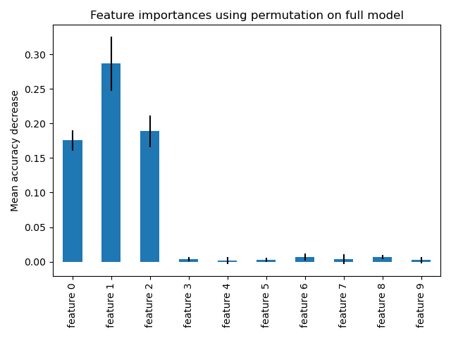
The same features are detected as most important using both methods. Although the relative importances vary. As seen on the plots, MDI is less likely than permutation importance to fully omit a feature.

Total running time of the script: ( 0 minutes 1.077 seconds)

Источник

3 Essential Ways to Calculate Feature Importance in Python

How can you find the most important features in your dataset? There’s a ton of techniques, and this article will teach you three any data scientist should know.

After reading, you’ll know how to calculate feature importance in Python with only a couple of lines of code. You’ll also learn the prerequisites of these techniques — crucial to making them work properly.

You can download the Notebook for this article here.

Dataset loading and preparation

Let’s spend as little time as possible here. You’ll use the Breast cancer dataset, which is built into Scikit-Learn. You’ll also need Numpy, Pandas, and Matplotlib for various analysis and visualization purposes.

The following snippet shows you how to import the libraries and load the dataset:

import numpy as np import pandas as pd from sklearn.datasets import load_breast_cancer  import matplotlib.pyplot as plt from matplotlib import rcParams rcParams['figure.figsize'] = 14, 7 rcParams['axes.spines.top'] = False rcParams['axes.spines.right'] = False  # Load data data = load_breast_cancer() 

The dataset isn’t in the most convenient format now. You’ll work with Pandas data frames most of the time, so let’s quickly convert it into one. The following snippet concatenates predictors and the target variable into a single data frame:

df = pd.concat([  pd.DataFrame(data.data, columns=data.feature_names),  pd.DataFrame(data.target, columns=['y']) ], axis=1)  df.head() 

Calling head() results in the following output:

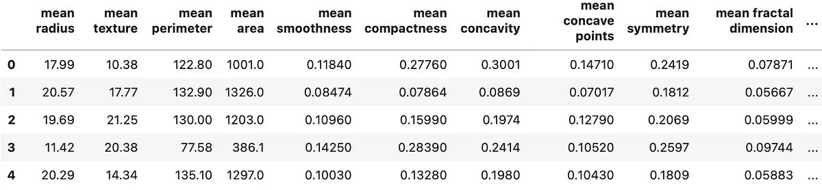
In a nutshell, there are 30 predictors and a single target variable. All of the values are numeric, and there are no missing values. The only obvious problem is the scale. Just take a look at the mean area and mean smoothness columns — the differences are drastic, which could result in poor models.

You’ll also need to perform a train/test split before addressing the scaling issue.

The following snippet shows you how to make a train/test split and scale the predictors with the StandardScaler class:

from sklearn.preprocessing import StandardScaler from sklearn.model_selection import train_test_split  X = df.drop('y', axis=1) y = df['y'] X_train, X_test, y_train, y_test = train_test_split(X, y, test_size=0.25, random_state=42)  ss = StandardScaler() X_train_scaled = ss.fit_transform(X_train) X_test_scaled = ss.transform(X_test) 

And that’s all you need to start obtaining feature importances. Let’s do that next.

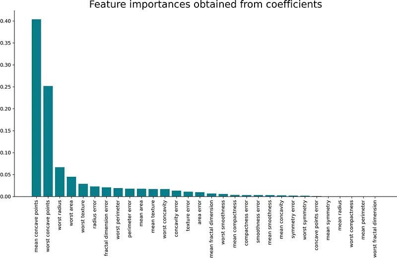
Method #1 — Obtain importances from coefficients

Probably the easiest way to examine feature importances is by examining the model’s coefficients. For example, both linear and logistic regression boils down to an equation in which coefficients (importances) are assigned to each input value.

Put simply, if an assigned coefficient is a large (negative or positive) number, it has some influence on the prediction. On the contrary, if the coefficient is zero, it doesn’t have any impact on the prediction.

Simple logic, but let’s put it to the test. We have a classification dataset, so logistic regression is an appropriate algorithm. After the model is fitted, the coefficients are stored in the coef_ property.

The following snippet trains the logistic regression model, creates a data frame in which the attributes are stored with their respective coefficients, and sorts that data frame by the coefficient in descending order:

from sklearn.linear_model import LogisticRegression  model = LogisticRegression() model.fit(X_train_scaled, y_train) importances = pd.DataFrame(data=  'Attribute': X_train.columns,  'Importance': model.coef_[0] >) importances = importances.sort_values(by='Importance', ascending=False) 

That was easy, wasn’t it? Let’s examine the coefficients visually next. The following snippet makes a bar chart from coefficients:

plt.bar(x=importances['Attribute'], height=importances['Importance'], color='#087E8B') plt.title('Feature importances obtained from coefficients', size=20) plt.xticks(rotation='vertical') plt.show() 

Here’s the corresponding visualization:

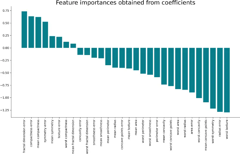
And that’s all there is to this simple technique. A take-home point is that the larger the coefficient is (in both positive and negative direction), the more influence it has on a prediction.

Method #2 — Obtain importances from a tree-based model

After training any tree-based models, you’ll have access to the feature_importances_ property. It’s one of the fastest ways you can obtain feature importances.

The following snippet shows you how to import and fit the XGBClassifier model on the training data. The importances are obtained similarly as before – stored to a data frame which is then sorted by the importance:

from xgboost import XGBClassifier  model = XGBClassifier() model.fit(X_train_scaled, y_train) importances = pd.DataFrame(data=  'Attribute': X_train.columns,  'Importance': model.feature_importances_ >) importances = importances.sort_values(by='Importance', ascending=False) 

You can examine the importance visually by plotting a bar chart. Here’s how to make one:

plt.bar(x=importances['Attribute'], height=importances['Importance'], color='#087E8B') plt.title('Feature importances obtained from coefficients', size=20) plt.xticks(rotation='vertical') plt.show() 

The corresponding visualization is shown below:

As mentioned earlier, obtaining importances in this way is effortless, but the results can come up a bit biased. The tendency of this approach is to inflate the importance of continuous features or high-cardinality categorical variables[1]. Make sure to do the proper preparation and transformations first, and you should be good to go.

Method #3 — Obtain importances from PCA loading scores

Principal Component Analysis (PCA) is a fantastic technique for dimensionality reduction, and can also be used to determine feature importance.

PCA won’t show you the most important features directly, as the previous two techniques did. Instead, it will return N principal components, where N equals the number of original features.

If you’re a bit rusty on PCA, there’s a complete from-scratch guide at the end of this article.

To start, let’s fit PCA to our scaled data and see what happens. The following snippet does just that and also plots a line plot of the cumulative explained variance:

from sklearn.decomposition import PCA  pca = PCA().fit(X_train_scaled)  plt.plot(pca.explained_variance_ratio_.cumsum(), lw=3, color='#087E8B') plt.title('Cumulative explained variance by number of principal components', size=20) plt.show() 

Here’s the corresponding visualization:

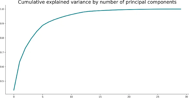
But what does this mean? It means you can explain 90-ish% of the variance in your source dataset with the first five principal components. Again, refer to the from-scratch guide if you don’t know what this means.

You can now start dealing with PCA loadings. These are just coefficients of the linear combination of the original variables from which the principal components are constructed[2]. You can use loadings to find correlations between actual variables and principal components.

If there’s a strong correlation between the principal component and the original variable, it means this feature is important — to say with the simplest words.

Here’s the snippet for computing loading scores with Python:

loadings = pd.DataFrame(  data=pca.components_.T * np.sqrt(pca.explained_variance_),  columns=[f'PCi>' for i in range(1, len(X_train.columns) + 1)],  index=X_train.columns ) loadings.head() 

The corresponding data frame looks like this:

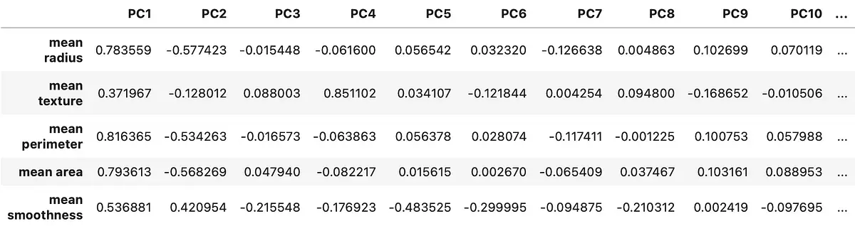
The first principal component is crucial. It’s just a single feature, but it explains over 60% of the variance in the dataset. As you can see from Image 5, the correlation coefficient between it and the mean radius feature is almost 0.8 — which is considered a strong positive correlation.

Let’s visualize the correlations between all of the input features and the first principal components. Here’s the entire code snippet (visualization included):

pc1_loadings = loadings.sort_values(by='PC1', ascending=False)[['PC1']] pc1_loadings = pc1_loadings.reset_index() pc1_loadings.columns = ['Attribute', 'CorrelationWithPC1']  plt.bar(x=pc1_loadings['Attribute'], height=pc1_loadings['CorrelationWithPC1'], color='#087E8B') plt.title('PCA loading scores (first principal component)', size=20) plt.xticks(rotation='vertical') plt.show() 

The corresponding visualization is shown below:

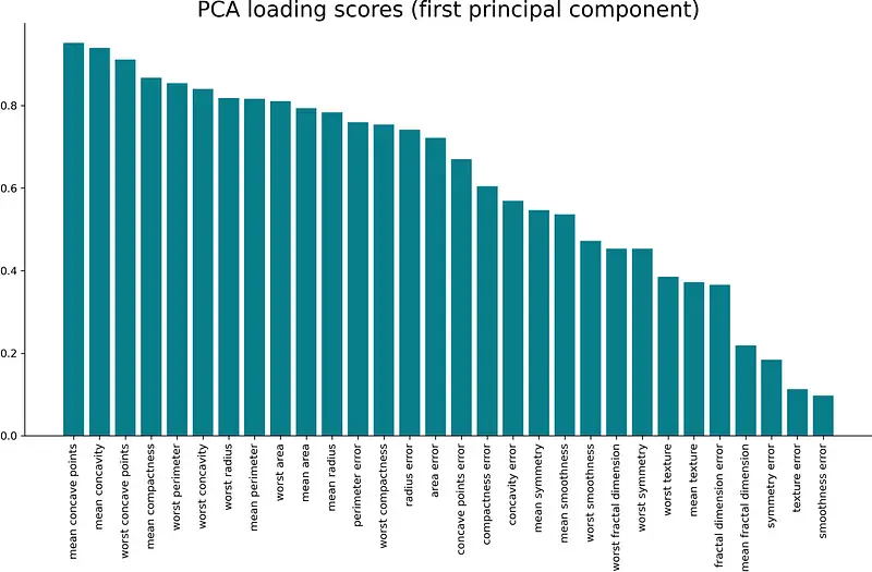
And that’s how you can “hack” PCA to use it as a feature importance algorithm. Let’s wrap things up in the next section.

Conclusion

And there you have it — three techniques you can use to find out what matters. Of course, there are many others, and you can find some of them in the Learn more section of this article.

These three should suit you well for any machine learning task. Just make sure to do the proper cleaning, exploration, and preparation first.

Learn More

Stay connected

Источник