3D Curve Fitting With Python
Curve fitting is a widely used technique in the field of data analysis and mathematical modeling. It involves the process of finding a mathematical function that best approximates a set of data points. In 3D curve fitting, the process is extended to three-dimensional space, where the goal is to find a function that best represents a set of 3D data points.
Python is a popular programming language used for scientific computing, and it provides several libraries that can be used for 3D curve fitting. In this article, we will discuss how to perform 3D curve fitting in Python using the SciPy library. so here In this article, we use how the SciPy library will be used for 3D curve fitting.
SciPy Library
The SciPy library is a powerful tool for scientific computing in Python. It provides a wide range of functionality for optimization, integration, interpolation, and curve fitting. In this article, we will focus on the curve-fitting capabilities of the library.
SciPy provides the curve_fit function, which can be used to perform curve fitting in Python. The function takes as input the data points to be fitted and the mathematical function to be used for fitting. The function then returns the optimized parameters for the mathematical function that best approximates the input data.
Let’s see the full step-by-step process for doing 3D Curve Fitting of 100 randomly generated points using the SciPy library in Python.
Prerequisites Library: here we use NumPy for generating random points and storing them, SciPy, and matplotlib for plotting these points in 3D space. so first of all install them using the below command in the terminal.
pip install numpy pip install scipy pip install matplotlib
3D Curve Fitting in Python
Let us now see how to perform 3D curve fitting in Python using the SciPy library. We will start by generating some random 3D data points using the NumPy library.
Python3
We have generated 100 random data points in 3D space, where the z-coordinate is defined as a function of the x and y coordinates with some added noise.
Next, we will define the mathematical function to be used for curve fitting. In this example, we will use a simple polynomial function of degree 3.
Python3
The function takes as input the x and y coordinates of a data point, and the six parameters a, b, c, d, e, and f. These parameters are the coefficients of the polynomial function that will be optimized during curve fitting.
We can now perform curve fitting using the curve_fit function from the SciPy library.
Python3
[ 0.04416919 -0.12960835 -0.11930051 0.16187097 0.1731539 0.85682108]
The curve_fit function takes as input the mathematical function to be used for curve fitting and the data points to be fitted. It returns two arrays, popt and pcov. The popt array contains the optimized values of the parameters of the mathematical function, and the pcov array contains the covariance matrix of the parameters.
The curve_fit() function in Python is used to perform nonlinear regression curve fitting. It uses the least-squares optimization method to find the optimized parameters of a user-defined function that best fit a given set of data.
About popt and pcov
popt and pcov are the two outputs of the curve_fit() function in Python. popt is a 1-D array of optimized parameters of the fitted function, while pcov is the estimated covariance matrix of the optimized parameters.
popt is calculated by minimizing the sum of squared residuals between the fitted function and the actual data points using a least-squares optimization algorithm. The curve_fit() function uses the Levenberg-Marquardt algorithm to perform this optimization. This algorithm iteratively adjusts the parameter values to minimize the objective function until convergence.
pcov is estimated using the covariance matrix of the gradient of the objective function at the optimized parameter values. The diagonal elements of pcov represent the variances of the optimized parameters, and the off-diagonal elements represent the covariances between the parameters. pcov is used to estimate the uncertainty in the optimized parameter values.
We can now use the optimized parameters to plot the fitted curve in 3D space.
SciPy Optimize Curve_fit
![]()
Python is a useful tool for fitting data to the desired functional form and is also used to calculate the standard error for any argument in a function fit. In Python, to find the best fit of data, and the optimal set of parameters for any user-defined function, the “curve_fit()” method can be used that enables flexibility.
In this guide, we will explain:
What is “SciPy” in Python?
The “SciPy” stands for “Scientific Python” which is the scientific computation open-source library and uses under the “NumPy”. It provides different utility functions for signal processing, stats, and optimization, such as “NumPy”.
What is “Optimize Curve_fit” in Python?
To get the best-fit parameter, the “Optimize Curve_fit” function can be used in Python. To obtain the optimized parameter for a provided function that fits the specified dataset, the “curve_fit()” function can be used. It is the freely available library in SciPy that is utilized to fit curves using the nonlinear least squares.it takes the input data, output data, and the desired function name that is to be employed.
How to Use Python’s “curve_fit” Function to Fit Data?
To fit any provided data set, first, import the required libraries, such as “numpy”, “matplotlib.pyplot”, “curve_fit”, and “warnings”. Then, specified the state of warning as “ignore”
import numpy as np
import matplotlib.pyplot as plt
from scipy.optimize import curve_fit
import warnings
warnings.filterwarnings ( ‘ignore’ )
Next, we have created the x-axis and y-axis values for a plot. Then, call an “np.asarray()” function and pass the previously created data to generate an array. After that, call the “plt.plot()” function with created arrays as parameters and the style of line in which we want to display the plot:
xaxis = [ — 5.0 , — 4.0 , — 3.0 , — 2.0 , — 1.0 , 0.0 , 1.0 , 2.0 , 3.0 , 4.0 , 5.0 ]
yaxis = [ 11.7 , 13.5 , 14.5 , 15.7 , 16.1 , 16.6 , 16.0 , 15.4 , 14.4 , 14.2 , 12.7 ]
xaxis = np.asarray ( xaxis )
yaxis = np.asarray ( yaxis )
plt.plot ( xaxis, yaxis, ‘o’ )
Now, we define the “Gaussian” function equation in Python to find the value of “M” and “N” that best fit our data. According to the below-provided code, this function will accept as inputs the x-axis values and all the arguments that will be best fit:
Next, call the “curve_fit()” function that takes the function that we need to fit, the values of the x-axis and y-axis as arguments. Then, the optimized values of the “M” and “N” are now saved in the list parameters:
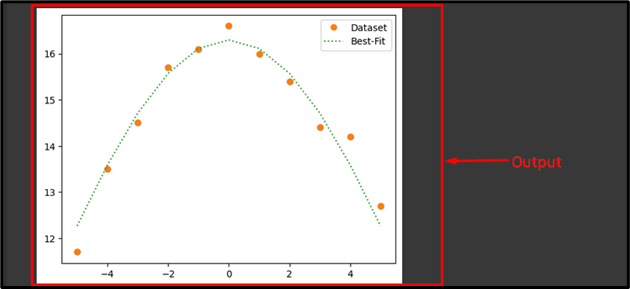
Now, we will calculate the values of the “y” by using our defined function and fit values of “M” and “N”. After that, create a plot to compare those calculated values to our specified data with the “label” parameter with value, function variables, and plot line style. Lastly, call the “plt.show” function to view the resultant plot:
fit_h = Gauss ( xaxis, fit_M, fit_N )
plt.plot ( xaxis, yaxis, ‘o’ , label = ‘Dataset’ )
plt.plot ( xaxis, fit_h, ‘:’ , label = ‘Best-Fit’ )
plt.legend ( )
plt.show ( )
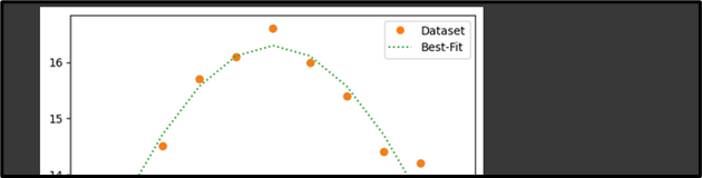
According to the provided output, we have found the best fit for our specified data:
That’s all! We have briefly explained the “curve_fit()” function in Python.
Conclusion
The “Optimize Curve_fit” function is used to get the best-fit parameter in Python and to obtain the optimized parameter for a provided function that fits the specified dataset, the “curve_fit()” function can be used. This guide elaborated on the SciPy Optimize Curve_fit in Python.
About the author
Maria Naz
I hold a master’s degree in computer science. I am passionate about my work, exploring new technologies, learning programming languages, and I love to share my knowledge with the world.