Бинаризация оцу opencv python

Содержание

Image Thresholding¶
Adaptive Thresholding¶
Otsu’s Binarization¶
How Otsu’s Binarization Works?¶
Бинаризация оцу opencv python
Adaptive Thresholding
Otsu’s Binarization
Бинаризация оцу opencv python
Adaptive Thresholding
Otsu’s Binarization

Image Thresholding¶

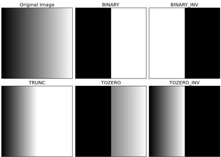
Here, the matter is straight forward. If pixel value is greater than a threshold value, it is assigned one value (may be white), else it is assigned another value (may be black). The function used is cv2.threshold. First argument is the source image, which should be a grayscale image. Second argument is the threshold value which is used to classify the pixel values. Third argument is the maxVal which represents the value to be given if pixel value is more than (sometimes less than) the threshold value. OpenCV provides different styles of thresholding and it is decided by the fourth parameter of the function. Different types are:

cv2.THRESH_BINARY
cv2.THRESH_BINARY_INV
cv2.THRESH_TRUNC
cv2.THRESH_TOZERO
cv2.THRESH_TOZERO_INV

Documentation clearly explain what each type is meant for. Please check out the documentation.

Two outputs are obtained. First one is a retval which will be explained later. Second output is our thresholded image.

import cv2 import numpy as np from matplotlib import pyplot as plt img = cv2.imread('gradient.png',0) ret,thresh1 = cv2.threshold(img,127,255,cv2.THRESH_BINARY) ret,thresh2 = cv2.threshold(img,127,255,cv2.THRESH_BINARY_INV) ret,thresh3 = cv2.threshold(img,127,255,cv2.THRESH_TRUNC) ret,thresh4 = cv2.threshold(img,127,255,cv2.THRESH_TOZERO) ret,thresh5 = cv2.threshold(img,127,255,cv2.THRESH_TOZERO_INV) titles = ['Original Image','BINARY','BINARY_INV','TRUNC','TOZERO','TOZERO_INV'] images = [img, thresh1, thresh2, thresh3, thresh4, thresh5] for i in xrange(6): plt.subplot(2,3,i+1),plt.imshow(images[i],'gray') plt.title(titles[i]) plt.xticks([]),plt.yticks([]) plt.show()

To plot multiple images, we have used plt.subplot() function. Please checkout Matplotlib docs for more details.

Adaptive Thresholding¶

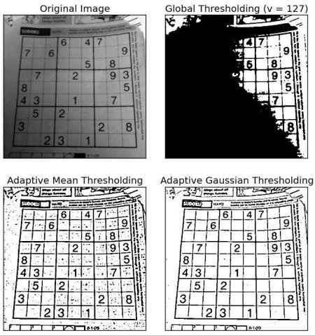
In the previous section, we used a global value as threshold value. But it may not be good in all the conditions where image has different lighting conditions in different areas. In that case, we go for adaptive thresholding. In this, the algorithm calculate the threshold for a small regions of the image. So we get different thresholds for different regions of the same image and it gives us better results for images with varying illumination.

It has three ‘special’ input params and only one output argument.

cv2.ADAPTIVE_THRESH_MEAN_C : threshold value is the mean of neighbourhood area.
cv2.ADAPTIVE_THRESH_GAUSSIAN_C : threshold value is the weighted sum of neighbourhood values where weights are a gaussian window.

Block Size — It decides the size of neighbourhood area.

C — It is just a constant which is subtracted from the mean or weighted mean calculated.

Below piece of code compares global thresholding and adaptive thresholding for an image with varying illumination:

import cv2 import numpy as np from matplotlib import pyplot as plt img = cv2.imread('dave.jpg',0) img = cv2.medianBlur(img,5) ret,th1 = cv2.threshold(img,127,255,cv2.THRESH_BINARY) th2 = cv2.adaptiveThreshold(img,255,cv2.ADAPTIVE_THRESH_MEAN_C,\ cv2.THRESH_BINARY,11,2) th3 = cv2.adaptiveThreshold(img,255,cv2.ADAPTIVE_THRESH_GAUSSIAN_C,\ cv2.THRESH_BINARY,11,2) titles = ['Original Image', 'Global Thresholding (v = 127)', 'Adaptive Mean Thresholding', 'Adaptive Gaussian Thresholding'] images = [img, th1, th2, th3] for i in xrange(4): plt.subplot(2,2,i+1),plt.imshow(images[i],'gray') plt.title(titles[i]) plt.xticks([]),plt.yticks([]) plt.show()

Otsu’s Binarization¶

In the first section, I told you there is a second parameter retVal. Its use comes when we go for Otsu’s Binarization. So what is it?

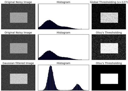
In global thresholding, we used an arbitrary value for threshold value, right? So, how can we know a value we selected is good or not? Answer is, trial and error method. But consider a bimodal image (In simple words, bimodal image is an image whose histogram has two peaks). For that image, we can approximately take a value in the middle of those peaks as threshold value, right ? That is what Otsu binarization does. So in simple words, it automatically calculates a threshold value from image histogram for a bimodal image. (For images which are not bimodal, binarization won’t be accurate.)

For this, our cv2.threshold() function is used, but pass an extra flag, cv2.THRESH_OTSU . For threshold value, simply pass zero. Then the algorithm finds the optimal threshold value and returns you as the second output, retVal . If Otsu thresholding is not used, retVal is same as the threshold value you used.

Check out below example. Input image is a noisy image. In first case, I applied global thresholding for a value of 127. In second case, I applied Otsu’s thresholding directly. In third case, I filtered image with a 5×5 gaussian kernel to remove the noise, then applied Otsu thresholding. See how noise filtering improves the result.

import cv2 import numpy as np from matplotlib import pyplot as plt img = cv2.imread('noisy2.png',0) # global thresholding ret1,th1 = cv2.threshold(img,127,255,cv2.THRESH_BINARY) # Otsu's thresholding ret2,th2 = cv2.threshold(img,0,255,cv2.THRESH_BINARY+cv2.THRESH_OTSU) # Otsu's thresholding after Gaussian filtering blur = cv2.GaussianBlur(img,(5,5),0) ret3,th3 = cv2.threshold(blur,0,255,cv2.THRESH_BINARY+cv2.THRESH_OTSU) # plot all the images and their histograms images = [img, 0, th1, img, 0, th2, blur, 0, th3] titles = ['Original Noisy Image','Histogram','Global Thresholding (v=127)', 'Original Noisy Image','Histogram',"Otsu's Thresholding", 'Gaussian filtered Image','Histogram',"Otsu's Thresholding"] for i in xrange(3): plt.subplot(3,3,i*3+1),plt.imshow(images[i*3],'gray') plt.title(titles[i*3]), plt.xticks([]), plt.yticks([]) plt.subplot(3,3,i*3+2),plt.hist(images[i*3].ravel(),256) plt.title(titles[i*3+1]), plt.xticks([]), plt.yticks([]) plt.subplot(3,3,i*3+3),plt.imshow(images[i*3+2],'gray') plt.title(titles[i*3+2]), plt.xticks([]), plt.yticks([]) plt.show()

Otsu

How Otsu’s Binarization Works?¶

This section demonstrates a Python implementation of Otsu’s binarization to show how it works actually. If you are not interested, you can skip this.

Since we are working with bimodal images, Otsu’s algorithm tries to find a threshold value (t) which minimizes the weighted within-class variance given by the relation :

$\sigma_w^2(t) = q_1(t)\sigma_1^2(t)+q_2(t)\sigma_2^2(t)$

$q_1(t) = \sum_</p data-lazy-src=$

^ P(i) \quad \& \quad q_1(t) = \sum_^ P(i) \mu_1(t) = \sum_^ \frac \quad \& \quad \mu_2(t) = \sum_^ \frac \sigma_1^2(t) = \sum_^ [i-\mu_1(t)]^2 \frac \quad \& \quad \sigma_2^2(t) = \sum_^ [i-\mu_1(t)]^2 \frac»/>

It actually finds a value of t which lies in between two peaks such that variances to both classes are minimum. It can be simply implemented in Python as follows:

img = cv2.imread('noisy2.png',0) blur = cv2.GaussianBlur(img,(5,5),0) # find normalized_histogram, and its cumulative distribution function hist = cv2.calcHist([blur],[0],None,[256],[0,256]) hist_norm = hist.ravel()/hist.max() Q = hist_norm.cumsum() bins = np.arange(256) fn_min = np.inf thresh = -1 for i in xrange(1,256): p1,p2 = np.hsplit(hist_norm,[i]) # probabilities q1,q2 = Q[i],Q[255]-Q[i] # cum sum of classes b1,b2 = np.hsplit(bins,[i]) # weights # finding means and variances m1,m2 = np.sum(p1*b1)/q1, np.sum(p2*b2)/q2 v1,v2 = np.sum(((b1-m1)**2)*p1)/q1,np.sum(((b2-m2)**2)*p2)/q2 # calculates the minimization function fn = v1*q1 + v2*q2 if fn  fn_min: fn_min = fn thresh = i # find otsu's threshold value with OpenCV function ret, otsu = cv2.threshold(blur,0,255,cv2.THRESH_BINARY+cv2.THRESH_OTSU) print thresh,ret

(Some of the functions may be new here, but we will cover them in coming chapters)

Additional Resources¶

Бинаризация оцу opencv python

Note To plot multiple images, we have used the plt.subplot() function. Please checkout the matplotlib docs for more details.

The code yields this result:

Adaptive Thresholding

In the previous section, we used one global value as a threshold. But this might not be good in all cases, e.g. if an image has different lighting conditions in different areas. In that case, adaptive thresholding can help. Here, the algorithm determines the threshold for a pixel based on a small region around it. So we get different thresholds for different regions of the same image which gives better results for images with varying illumination.

In addition to the parameters described above, the method cv.adaptiveThreshold takes three input parameters:

The adaptiveMethod decides how the threshold value is calculated:

cv.ADAPTIVE_THRESH_MEAN_C: The threshold value is the mean of the neighbourhood area minus the constant C.
cv.ADAPTIVE_THRESH_GAUSSIAN_C: The threshold value is a gaussian-weighted sum of the neighbourhood values minus the constant C.

The blockSize determines the size of the neighbourhood area and C is a constant that is subtracted from the mean or weighted sum of the neighbourhood pixels.

The code below compares global thresholding and adaptive thresholding for an image with varying illumination:

Otsu’s Binarization

In global thresholding, we used an arbitrary chosen value as a threshold. In contrast, Otsu’s method avoids having to choose a value and determines it automatically.

Consider an image with only two distinct image values (bimodal image), where the histogram would only consist of two peaks. A good threshold would be in the middle of those two values. Similarly, Otsu’s method determines an optimal global threshold value from the image histogram.

In order to do so, the cv.threshold() function is used, where cv.THRESH_OTSU is passed as an extra flag. The threshold value can be chosen arbitrary. The algorithm then finds the optimal threshold value which is returned as the first output.

Check out the example below. The input image is a noisy image. In the first case, global thresholding with a value of 127 is applied. In the second case, Otsu’s thresholding is applied directly. In the third case, the image is first filtered with a 5×5 gaussian kernel to remove the noise, then Otsu thresholding is applied. See how noise filtering improves the result.

Источник