Augmented Reality using ArUco Markers in OpenCV (C++ / Python)
In this post, we will explain what ArUco markers are and how to use them for simple augmented reality tasks using OpenCV.
ArUco markers have been used for a while in augmented reality, camera pose estimation, and camera calibration. Let’s learn more about them.
What are ArUco markers?
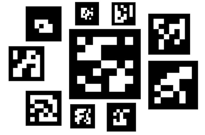
ArUco markers were originally developed in 2014 by S.Garrido-Jurado et al., in their work “Automatic generation and detection of highly reliable fiducial markers under occlusion“. ArUco stands for Augmented Reality University of Cordoba. That is where it was developed in Spain. Below are some examples of the ArUco markers.
An aruco marker is a fiducial marker that is placed on the object or scene being imaged. It is a binary square with black background and boundaries and a white generated pattern within it that uniquely identifies it. The black boundary helps making their detection easier. They can be generated in a variety of sizes. The size is chosen based on the object size and the scene, for a successful detection. If very small markers are not being detected, just increasing their size can make their detection easier.
The idea is that you print these markers and put them in the real world. You can photograph the real world and detect these markers uniquely.
If you are a beginner, you may be thinking how is this useful? Let’s look at a couple of use cases.
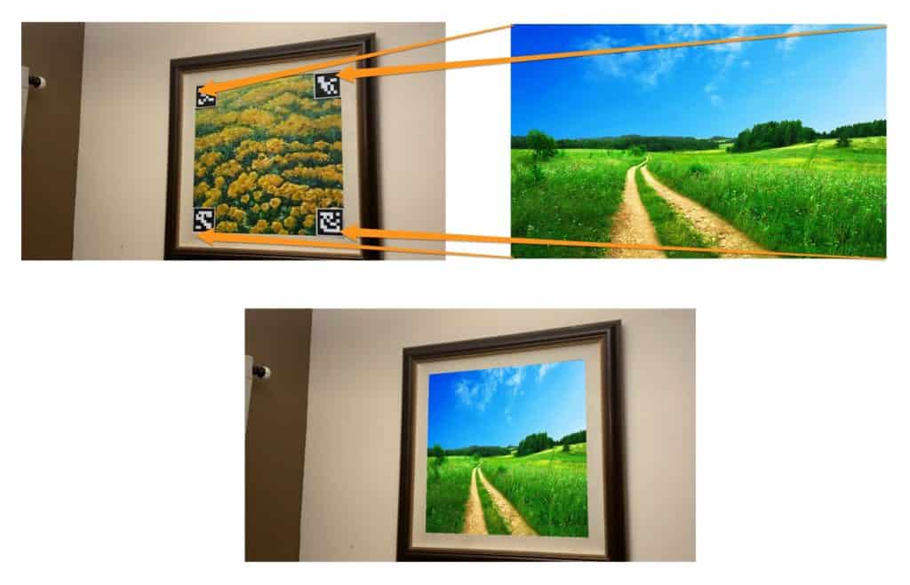
In the example we have shared in the post, we have put the printed and put the markers on the corners of a picture frame. When we uniquely identify the markers, we are able to replace the picture frame with an arbitrary video or image. The new picture has the correct perspective distortion when we move the camera.
In a robotics application, you can put these markers along the path of the warehouse robot equipped with a camera. When the camera mounted on the robot detects one these markers, it can know its precise location in the warehouse because each marker has a unique ID and we know where the markers were placed in the warehouse.
Generating ArUco markers in OpenCV
We can generate these markers very easily using OpenCV. The aruco module in OpenCV has a total of 25 predefined dictionaries of markers. All the markers in a dictionary contain the same number of blocks or bits(4×4, 5×5, 6×6 or 7×7), and each dictionary contains a fixed number of markers(50, 100, 250 or 1000). Below we show how to generate and detect various kinds of aruco markers in both C++ and Python.
We will need to use the aruco module in the code.
The function call getPredefinedDictionary below shows how to load a dictionary of 250 markers, where each marker contains a 6×6 bit binary pattern.
Download Code To easily follow along this tutorial, please download code by clicking on the button below. It’s FREE!
C++
// Import the aruco module in OpenCV #include Mat markerImage; // Load the predefined dictionary Ptr dictionary = aruco::getPredefinedDictionary(cv::aruco::DICT_6X6_250); // Generate the marker aruco::drawMarker(dictionary, 33, 200, markerImage, 1);
Python
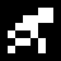
import cv2 as cv import numpy as np # Load the predefined dictionary dictionary = cv.aruco.Dictionary_get(cv.aruco.DICT_6X6_250) # Generate the marker markerImage = np.zeros((200, 200), dtype=np.uint8) markerImage = cv.aruco.drawMarker(dictionary, 33, 200, markerImage, 1); cv.imwrite("marker33.png", markerImage); The drawMarker function above lets us choose the marker with a given id (the second parameter – 33) from the collection of 250 markers which have ids from 0 to 249. The third parameter to the drawMarker function decides the size of the marker generated. In the above example, it would generate an image with 200×200 pixels. The fourth parameter represents the object that would store the generated marker (markerImage above). Finally, the fifth parameter is the thickness parameter and decides how many blocks should be added as boundary to the generated binary pattern. In the above example, a boundary of 1 bit would be added around the 6×6 generated pattern, to produce an image with 7×7 bits in a 200×200 pixel image. The marker generated using the above code would look like the image below.
For most applications, we need to generate multiple markers, print them and put in the scene.
Detecting Aruco markers
Once the scene is imaged with the aruco markers, we need to detect them and use them for further processing. Below we show how to detect the markers.
C++
// Load the dictionary that was used to generate the markers. Ptr dictionary = getPredefinedDictionary(DICT_6X6_250); // Initialize the detector parameters using default values Ptr parameters = DetectorParameters::create(); // Declare the vectors that would contain the detected marker corners and the rejected marker candidates vector> markerCorners, rejectedCandidates; // The ids of the detected markers are stored in a vector vector markerIds; // Detect the markers in the image detectMarkers(frame, dictionary, markerCorners, markerIds, parameters, rejectedCandidates);
Python
#Load the dictionary that was used to generate the markers. dictionary = cv.aruco.Dictionary_get(cv.aruco.DICT_6X6_250) # Initialize the detector parameters using default values parameters = cv.aruco.DetectorParameters_create() # Detect the markers in the image markerCorners, markerIds, rejectedCandidates = cv.aruco.detectMarkers(frame, dictionary, parameters=parameters)
We start by loading the same dictionary that we used to generate the markers.
An initial set of parameters are detected using DetectorParameters::create(). OpenCV allows us to change multiple parameters in the detection process. The list of parameters that can be adjusted including the adaptive threshold values can be found here. In most of the cases, the default parameter work well and OpenCV recommends to use those. So we will stick to the default parameters.
For each successful marker detection, the four corner points of the marker are detected, in order from top left, top right, bottom right and bottom left. In C++, these 4 detected corner points are stored as a vector of points and multiple markers in the image are together stored in a vector of vector of points. In Python, they are stored as Numpy array of arrays.
The detectMarkers function is used to detect and locate the corners of the markers. The first parameter is the image of the scene with the markers. The second parameter is the dictionary used to generate the markers. The successfully detected markers will be stored in markerCorners and their ids are stored in markerIds . The DetectorParameters object initialized earlier is also passed as a parameter. Finally, the rejected candidates are stored in rejectedCandidates .
While printing, cutting and placing the markers in a scene, it is important that we retain some white border around the marker’s black boundary, so that they can be detected easily.
Master Generative AI for CV
Get expert guidance, insider tips & tricks. Create stunning images, learn to fine tune diffusion models, advanced Image editing techniques like In-Painting, Instruct Pix2Pix and many more
An Augmented Reality Application
The ArUco markers were primarily developed to solve the problem of camera pose estimation for various applications including augmented reality. OpenCV elaborately describes the pose estimation process in its documentation.
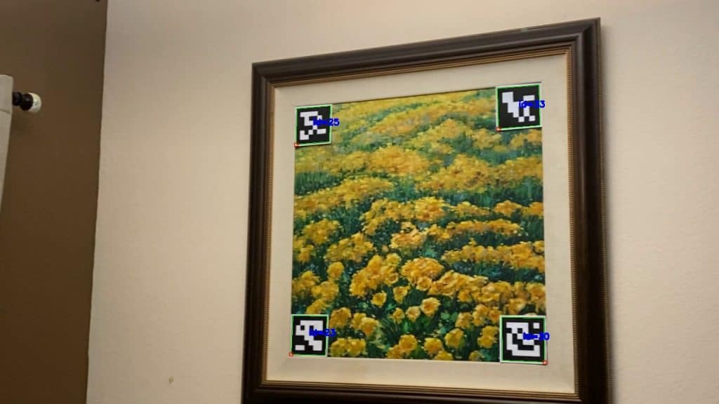
In this post, we will use them for an augmented reality application which lets us overlay any new scene onto an existing image or video. We pick a scene at home with a large picture frame, and we want to replace the picture in the frame by new ones to see how they look up on the wall. We then go ahead and try to insert a video in a movie. For this purpose, we print, cut and paste large aruco markers onto the corners of image area as seen in the picture below, and then capture the video. The captured video is in the left part of the video at the top of the post. We then process each frame of the video individually in order.
For each image, the markers are first detected. The picture below shows the detected markers drawn in the green. The first point is marked with a small red circle. The second, third and fourth points can be accessed by traversing the border of the marker clockwise.
Four corresponding set of points in the input image and the new scene image are used to compute a homography. We explained homography in one of our earlier posts here. Given corresponding points in different views of a scene, homography is a transform that maps one corresponding point to another.
In our case, the homography matrix is used to warp the new scene image into the quadrilateral defined by the markers in our captured image. We show how to do that in the code below.
C++
// Compute homography from source and destination points Mat h = cv::findHomography(pts_src, pts_dst); // Warped image Mat warpedImage; // Warp source image to destination based on homography warpPerspective(im_src, warpedImage, h, frame.size(), INTER_CUBIC); // Prepare a mask representing region to copy from the warped image into the original frame. Mat mask = Mat::zeros(frame.rows, frame.cols, CV_8UC1); fillConvexPoly(mask, pts_dst, Scalar(255, 255, 255)); // Erode the mask to not copy the boundary effects from the warping Mat element = getStructuringElement( MORPH_RECT, Size(3,3) ); erode(mask, mask, element); // Copy the masked warped image into the original frame in the mask region. Mat imOut = frame.clone(); warpedImage.copyTo(imOut, mask);
Python
# Calculate Homography h, status = cv.findHomography(pts_src, pts_dst) # Warp source image to destination based on homography warped_image = cv.warpPerspective(im_src, h, (frame.shape[1],frame.shape[0])) # Prepare a mask representing region to copy from the warped image into the original frame. mask = np.zeros([frame.shape[0], frame.shape[1]], dtype=np.uint8); cv.fillConvexPoly(mask, np.int32([pts_dst_m]), (255, 255, 255), cv.LINE_AA); # Erode the mask to not copy the boundary effects from the warping element = cv.getStructuringElement(cv.MORPH_RECT, (3,3)); mask = cv.erode(mask, element, iterations=3); # Copy the mask into 3 channels. warped_image = warped_image.astype(float) mask3 = np.zeros_like(warped_image) for i in range(0, 3): mask3[. i] = mask/255 # Copy the masked warped image into the original frame in the mask region. warped_image_masked = cv.multiply(warped_image, mask3) frame_masked = cv.multiply(frame.astype(float), 1-mask3) im_out = cv.add(warped_image_masked, frame_masked)
We use the new scene image corner points as the source points(pts_src), and corresponding picture corner points inside the picture frame in our captured image as the destination points(dst_src). The OpenCV function findHomography computes the homography function h between the source and destination points. The homography matrix is then used to warp the new image to fit into the target frame. The warped image is masked and copied into the target frame. In case of video, this process is repeated on each frame.
Subscribe & Download Code
If you liked this article and would like to download code (C++ and Python) and example images used in this post, please click here. Alternately, sign up to receive a free Computer Vision Resource Guide. In our newsletter, we share OpenCV tutorials and examples written in C++/Python, and Computer Vision and Machine Learning algorithms and news.


